Feeds:
Posts
Comments

Archive for the ‘Value Investment’ Category

Aswath Damodaran, a Professor of Finance at the Stern School of Business, has an interesting post on his blog Musings on Markets, Transaction costs and beating the market. Damodaran’s thesis is that transaction costs – broadly defined to include brokerage commissions, spread and the “price impact” of trading (which I believe is an important issue for some strategies) – foil in the real world investment strategies that beat the market in back-tests. He argues that transaction costs are also the reason why the “average active portfolio manager” underperforms the index by about 1% to 1.5%. I agree with Damodaran. The long-term, successful practical application of any investment strategy is difficult, and is made more so by all of the frictional costs that the investor encounters. That said, I see no reason why a systematic application of some value-based investment strategies should not outperform the market even after taking into account those transaction costs and taxes. That’s a bold statement, and requires in support the production of equally extraordinary evidence, which I do not possess. Regardless, here’s my take on Damodaran’s article.

First, Damodaran makes the point that even well-researched, back-tested, market-beating strategies underperform in practice:

Most of these beat-the-market approaches, and especially the well researched ones, are backed up by evidence from back testing, where the approach is tried on historical data and found to deliver “excess returns”. Ergo, a money making strategy is born.. books are written.. mutual funds are created.

The average active portfolio manager, who I assume is the primary user of these can’t-miss strategies does not beat the market and delivers about 1-1.5% less than the index. That number has remained surprisingly stable over the last four decades and has persisted through bull and bear markets. Worse, this under performance cannot be attributed to “bad” portfolio mangers who drag the average down, since there is very little consistency in performance. Winners this year are just as likely to be losers next year…

Then he explains why he believes market-beating strategies that work on paper fail in the real world. The answer? Transaction costs:

So, why do portfolios that perform so well in back testing not deliver results in real time? The biggest culprit, in my view, is transactions costs, defined to include not only the commission and brokerage costs but two more significant costs – the spread between the bid price and the ask price and the price impact you have when you trade. The strategies that seem to do best on paper also expose you the most to these costs. Consider one simple example: Stocks that have lost the most of the previous year seem to generate much better returns over the following five years than stocks have done the best. This “loser” stock strategy was first listed in the academic literature in the mid-1980s and greeted as vindication by contrarians. Later analysis showed, though, that almost all of the excess returns from this strategy come from stocks that have dropped to below a dollar (the biggest losing stocks are often susceptible to this problem). The bid-ask spread on these stocks, as a percentage of the stock price, is huge (20-25%) and the illiquidity can also cause large price changes on trading – you push the price up as you buy and the price down as you sell. Removing these stocks from your portfolio eliminated almost all of the excess returns.

In support of his thesis, Damodaran gives the example of Value Line and its mutual funds:

In perhaps the most telling example of slips between the cup and lip, Value Line, the data and investment services firm, got great press when Fischer Black, noted academic and believer in efficient markets, did a study where he indicated that buying stocks ranked 1 in the Value Line timeliness indicator would beat the market. Value Line, believing its own hype, decided to start mutual funds that would invest in its best ranking stocks. During the years that the funds have been in existence, the actual funds have underperformed the Value Line hypothetical fund (which is what it uses for its graphs) significantly.

Damodaran’s argument is particularly interesting to me in the context of my recent series of posts on quantitative value investing. For those new to the site, my argument is that a systematic application of the deep value methodologies like Benjamin Graham’s liquidation strategy (for example, as applied in Oppenheimer’s Ben Graham’s Net Current Asset Values: A Performance Update) or a low price-to-book strategy (as described in Lakonishok, Shleifer, and Vishny’s Contrarian Investment, Extrapolation and Risk) can lead to exceptional long-term investment returns in a fund.

When Damodaran refers to “the price impact you have when you trade” he highlights a very important reason why a strategy in practice will underperform its theoretical results. As I noted in my conclusion to Intuition and the quantitative value investor:

The challenge is making the sample mean (the portfolio return) match the population mean (the screen). As we will see, the real world application of the quantitative approach is not as straight-forward as we might initially expect because the act of buying (selling) interferes with the model.

A strategy in practice will underperform its theoretical results for two reasons:

  1. The strategy in back test doesn’t have to deal with what I call the “friction” it encounters in the real world. I define “friction” as brokerage, spread and tax, all of which take a mighty bite out of performance. These are two of Damodaran’s transaction costs and another – tax. Arguably spread is the most difficult to prospectively factor into a model. One can account for brokerage and tax in the model, but spread is always going to be unknowable before the event.
  2. The act of buying or selling interferes with the market (I think it’s a Schrodinger’s cat-like paradox, but then I don’t understand quantum superpositions). This is best illustrated at the micro end of the market. Those of us who traffic in the Graham sub-liquidation value boat trash learn to live with wide spreads and a lack of liquidity. We use limit orders and sit on the bid (ask) until we get filled. No-one is buying (selling) “at the market,” because, for the most part, there ain’t no market until we get on the bid (ask). When we do manage to consummate a transaction, we’re affecting the price. We’re doing our little part to return it to its underlying value, such is the wonderful phenomenon of value investing mean reversion in action. The back-test / paper-traded strategy doesn’t have to account for the effect its own buying or selling has on the market, and so should perform better in theory than it does in practice.

If ever the real-world application of an investment strategy should underperform its theoretical results, Graham liquidation value is where I would expect it to happen. The wide spreads and lack of liquidity mean that even a small, individual investor will likely underperform the back-test results. Note, however, that it does not necessarily follow that the Graham liquidation value strategy will underperform the market, just the model. I continue to believe that a systematic application of Graham’s strategy will beat the market in practice.

I have one small quibble with Damodaran’s otherwise well-argued piece. He writes:

The average active portfolio manager, who I assume is the primary user of these can’t-miss strategies does not beat the market and delivers about 1-1.5% less than the index.

There’s a little rhetorical sleight of hand in this statement (which I’m guilty of on occasion in my haste to get a post finished). Evidence that the “average active portfolio manager” does not beat the market is not evidence that these strategies don’t beat the market in practice. I’d argue that the “average active portfolio manager” is not using these strategies. I don’t really know what they’re doing, but I’d guess the institutional imperative calls for them to hug the index and over- or under-weight particular industries, sectors or companies on the basis of a story (“Green is the new black,” “China will consume us back to the boom,” “house prices never go down,” “the new dot com economy will destroy the old bricks-and-mortar economy” etc). Yes, most portfolio managers underperform the index in the order of 1% to 1.5%, but I think they do so because they are, in essence, buying the index and extracting from the index’s performance their own fees and other transaction costs. They are not using the various strategies identified in the academic or popular literature. That small point aside, I think the remainder of the article is excellent.

In conclusion, I agree with Damodaran’s thesis that transaction costs in the form of brokerage commissions, spread and the “price impact” of trading make many apparently successful back-tested strategies unusable in the real world. I believe that the results of any strategy’s application in practice will underperform its theoretical results because of friction and the paradox of Schrodinger’s cat’s brokerage account. That said, I still see no reason why a systematic application of Graham’s liquidation value strategy or LSV’s low price-to-book value strategy can’t outperform the market even after taking into account these frictional costs and, in particular, wide spreads.

Hat tip to the Ox.

Read Full Post »

In his Are Japanese equities worth more dead than alive?, SocGen’s Dylan Grice conducted some research into the performance of sub-liquidation value stocks in Japan since the mid 1990s. Grice’s findings are compelling:

My Factset backtest suggests such stocks trading below liquidation value have averaged a monthly return of 1.5% since the mid 1990s, compared to -0.2% for the Topix. There is no such thing as a toxic asset, only a toxic price. It may well be that these companies have no future, that they shouldn’t be valued as going concerns and that they are worth more dead than alive. If so, they are already trading at a value lower than would be fetched in a fire sale. But what if the outlook isn’t so gloomy? If these assets aren’t actually complete duds, we could be looking at some real bargains…

In the same article, Grice identifies five Graham net net stocks in Japan with market capitalizations bigger than $1B:

He argues that such stocks may offer value beyond the net current asset value:

The following chart shows the debt to shareholders equity ratios for each of the stocks highlighted as a liquidation candidate above, rebased so that the last year’s number equals 100. It’s clear that these companies have been aggressively delivering in the last decade.

Despite the “Japan has weak shareholder rights” cover story, management seems to be doing the right thing:

But as it happens, most of these companies have also been buying back stock too. So per share book values have been rising steadily throughout the appalling macro climate these companies have found themselves in. Contrary to what I expected to find, these companies that are currently priced at levels making liquidation seem the most profitable option have in fact been steadily creating shareholder wealth.

This is really extraordinary. The currency is a risk that I can’t quantify, but it warrants further investigation.

Read Full Post »

Since last week’s Japanese liquidation value: 1932 US redux post, I’ve been attempting to determine whether the historical performance of Japanese sub-liquidation value stocks matches the experience in the US, which has been outstanding since the strategy was first identified by Benjamin Graham in 1932. The risk to the Japanese net net experience is the perception (rightly or not) that the weakness of shareholder rights in Japan means that net current asset value stocks there are destined to continue to trade at a discount to net current asset value. As I mentioned yesterday, I’m a little chary of the “Japan has weak shareholder rights” narrative. I’d rather look at the data, but the data are a little wanting.

As we all know, the US net net experience has been very good. Research undertaken by Professor Henry Oppenheimer on Graham’s liquidation value strategy between 1970 and 1983, published in the paper Ben Graham’s Net Current Asset Values: A Performance Update, indicates that “[the] mean return from net current asset stocks for the 13-year period was 29.4% per year versus 11.5% per year for the NYSE-AMEX Index. One million dollars invested in the net current asset portfolio on December 31, 1970 would have increased to $25,497,300 by December 31, 1983.” That’s an outstanding return.

In The performance of Japanese common stocks in relation to their net current asset values, a 1993 paper by Bildersee, Cheh and Zutshi, the authors undertook research similar to Oppenheimer’s in Japan over the period 1975 and 1988. Their findings, described in another paper, indicate that the Japanese net net investor’s experience has not been as outstanding as the US investor’s:

In the first study outside of the USA, Bildersee, Cheh and Zutshi (1993)’s paper focuses on the Japanese market from 1975 to 1988. In order to maintain a sample large enough for cross-sectional analysis, Graham’s criterion was relaxed so that firms are required to merely have an NCAV/MV ratio greater than zero. They found the mean market-adjusted return of the aggregate portfolio is around 1 percent per month (13 percent per year).

As an astute reader noted last week “…the test period for [the Bildersee] study is not the best. It includes Japan’s best analog to America’s Roaring Twenties. The Nikkei peaked on 12/29/89, and never recovered:”

Many of the “assets” on public companies’ books at that time were real estate bubble-related. At the peak in 1989, the aggregate market price for all private real estate in the city of Tokyo was purportedly greater than that of the entire state of California. You can see how the sudden runup in real estate during the bubble could cause asset-heavy companies to outperform the market.

So a better crucible for Japanese NCAVs might be the deflationary period, say beginning 1/1/90, which is more analogous to the US in 1932.

To see how the strategy has performed more recently, I’ve taken the Japanese net net stocks identified in James Montier’s Graham’’s net-nets: outdated or outstanding? article from September 2008 and tracked their performance from the data of the article to today. Before I plow into the results, I’d like to discuss my methodology and the various problems with it:

  1. It was not possible to track all of the stocks identified by Montier. Where I couldn’t find a closing price for a stock, I’ve excluded it from the results and marked the stock as “N/A”. I’ve had to exclude 18 of 84 stocks, which is a meaningful proportion. It’s possible that these stocks were either taken over or went bust, and so would have had an effect on the results not reflected in my results.
  2. The opening prices were not always available. In some instances I had to use the price on another date close to the opening date (i.e +/1 month).

Without further ado, here are the results of Montier’s Graham’’s net-nets: outdated or outstanding? picks:

The 68 stocks tracked gained on average 0.5% between September 2008 and February 2010, which is a disappointing outcome. The results relative to the  Japanese index are a little better. By way of comparison, the Nikkei 225 (roughly equivalent to the DJIA) fell from 12,834 to close yesterday at 10,057, a drop of 21.6%. Encouragingly, the net nets outperformed the N225 by a little over 21%.

The paucity of the data is a real problem for this study. I’ll update this post as I find more complete data or a more recent study.

Read Full Post »

Mariusz Skonieczny is the founder and president of Classic Value Investors LLC and runs the Classic Value Investors website. He has provided me with a copy of his book Why Are We So Clueless about the Stock Market? Learn How to Invest Your Money, How to Pick Stocks, and How to Make Money in the Stock Market and has asked me to review it for the site. I am happy to do so.

Mariusz says that the purpose of this book is to “help readers understand the basics of stock market investing:”

Material covered includes the difference between stocks and businesses, what constitutes a good business, when to buy and sell stocks, and how to value individual stocks. The book also includes a chapter covering four case studies as well as a supplemental chapter on the pros and cons of real estate versus stock market investing.

The book discusses the basics of valuation through return on equity, how to identify a “good” businesses with sustainable competitive advantages (moats), diversification, how to understand the capital structure, and the implications of the economy for the business analyzed. Most usefully, Mariusz also discusses how to analyze an investment and provides several case studies discussing his methodology. In my opinion, the book is an excellent introduction to Buffett-style investing, and I would recommend it to investors seeking “wonderful companies at a fair price.”

Read Full Post »

In “Black box” blues I argued that automated trading was a potentially dangerous element to include in a quantitative investment strategy, citing the “program trading / portfolio insurance” crash of 1987. When the market started falling in 1987 the computer programs caused the writers of derivatives to sell on every down-tick, which some suggest exacerbated the crash. Here’s New York University’s Richard Sylla discussing the causes (care of Wikipedia).

The internal reasons included innovations with index futures and portfolio insurance. I’ve seen accounts that maybe roughly half the trading on that day was a small number of institutions with portfolio insurance. Big guys were dumping their stock. Also, the futures market in Chicago was even lower than the stock market, and people tried to arbitrage that. The proper strategy was to buy futures in Chicago and sell in the New York cash market. It made it hard — the portfolio insurance people were also trying to sell their stock at the same time.

The Economist’s Buttonwood column has an article, Model behaviour: The drawbacks of automated trading, which argues along the same lines that automated trading is potentially problematic where too many managers follow the same approach:

[If] you feed the same data into computers in search of anomalies, they are likely to come up with similar answers. This can lead to some violent market lurches.

Buttonwood divides the quantitative approaches to investing into at three different types and their potential for providing a stabilizing influence on the market or throwing fuel on the fire in a crash:

1. Trend-following, the basis of which is that markets have “momentum”:

The model can range across markets and go short (bet on falling prices) as well as long, so the theory is that there will always be some kind of trend to exploit. A paper by AQR, a hedge-fund group, found that a simple trend-following system produced a 17.8% annual return over the period from 1985 to 2009. But such systems are vulnerable to turning-points in the markets, in which prices suddenly stop rising and start to fall (or vice versa). In late 2009 the problem for AHL seemed to be that bond markets and currencies, notably the dollar, seemed to change direction.

2. Value, which seeks securities that are  cheap according to “a specific set of criteria such as dividend yields, asset values and so on:”

The value effect works on a much longer time horizon than momentum, so that investors using those models may be buying what the momentum models are selling. The effect should be to stabilise markets.

3.  Arbitrage, which exploits price differentials between securities where no such price differential should exist:

This ceaseless activity, however, has led to a kind of arms race in which trades are conducted faster and faster. Computers now try to take advantage of arbitrage opportunities that last milliseconds, rather than hours. Servers are sited as close as possible to stock exchanges to minimise the time taken for orders to travel down the wires.

In arguing that automated trading can be problematic where too many managers pursue the same strategy, Buttonwood gives the example of the August 2007 crash, which sounds eerily similar to Sylla’s explanation for the 1987 crash above:

A previous example occurred in August 2007 when a lot of them got into trouble at the same time. Back then the problem was that too many managers were following a similar approach. As the credit crunch forced them to cut their positions, they tried to sell the same shares at once. Prices fell sharply and portfolios that were assumed to be well-diversified turned out to be highly correlated.

It is interesting that over-crowding is the same problem identified by GSAM in Goldman Claims Momentum And Value Quant Strategies Now Overcrowded, Future Returns Negligible. In that presentation, Robert Litterman, Goldman Sachs’ Head of Quantitative Resources, said:

Computer-driven hedge funds must hunt for new areas to exploit as some areas of making money have become so overcrowded they may no longer be profitable, according to Goldman Sachs Asset Management. Robert Litterman, managing director and head of quantitative resources, said strategies such as those which focus on price rises in cheaply-valued stocks, which latch onto market momentum or which trade currencies, had become very crowded.

Litterman argued that only special situations and event-driven strategies that focus on mergers or restructuring provide opportunities for profit (perhaps because these strategies require human judgement and interaction):

What we’re going to have to do to be successful is to be more dynamic and more opportunistic and focus especially on more proprietary forecasting signals … and exploit shorter-term opportunistic and event-driven types of phenomenon.

As we’ve seen before, human judgement is often flawed. Buttonwood says:

Computers may not have the human frailties (like an aversion to taking losses) that traditional fund managers display. But turning the markets over to the machines will not necessarily make them any less volatile.

And we’ve come full circle: Human’s are flawed, computers are the answer. Computers are flawed, humans are the answer. How to break the deadlock? I think it’s time for Taleb’s skeptical empiricist to emerge. More to come.

Read Full Post »

Recently I’ve been laying the groundwork for a quantitative approach to value investment. The rational is as follows: simple quantitative or statistical models outperform experts in a variety of disciplines, so why not investing in general, and why not value investing in specific? Well, it seems that they do. A new research paper argues that quantitative funds outperform their qualitative brethren. In A Comparison of Quantitative and Qualitative Hedge Funds (via CXO Advisory Group blog) Ludwig Chincarini has compared the performance characteristics of quantitative and qualitative hedge funds. Chincarini finds that “both quantitative and qualitative hedge funds have positive risk-adjusted returns,” but, “overall, quantitative hedge funds as a group have higher [alpha] than qualitative hedge funds.”

Definition of quantitative and qualitative

Chincarini distinguished between quantitative and qualitative equity-focussed funds thus:

Our main method used to classify was to look for the term quantitative or a description of a similar nature to place a fund in the quantative category. We also looked for words like discretionary to classify qualitative funds and systematic to classify quantitative funds. Of the four main hedge fund categories, we only found two of them reliable enough to classify. Thus, in the Equity Hedge category, we classified Equity Market Neutral and Quantitative Directional as quantitative hedge funds and Fundamental Growth and Fundamental Value as qualitative categories.

We did not classify any of the Event Driven funds since these funds vary too substantially within the category and it was not clear from the descriptions how to separate quantitative and qualitative funds. We also did not classify any of the Relative Value funds, even though many of these funds use quantitative techniques, because the broader descriptions left us no clear cut way to divide them.

We classified a fund as quantitative if the following words appeared in the fund description: quantitative, mathematical, model, algorithm, econometric, statistic, or automate. Also, the fund description could not contain the word qualitative. We classified a fund as qualitative if it contained the word qualitative in its description or had none of the words mentioned for the quantitative category.

Performance

Using return data from 6,354 hedge funds from January 1970 through June 2009, Cincarini concludes, based on the raw performance data:

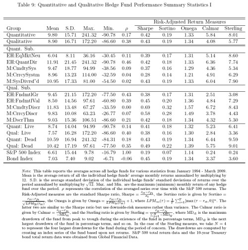
Generally, quantitative funds have a higher average return and a lower average standard deviation than qual funds. Amongst the quant funds, the highest average return comes from the Quantitative Directional strategy. The correlations of the fund categories with the S&P 500 are quite low at 0.17 and 0.38 for quant and qual respectively. The risk-adjusted return measures provide mixed evidence, but overall seems in favor of quant funds.

The qual funds perform significantly better than quant funds in up markets (25% and 15% respectively). However, the quant funds do significantly better in down markets (-2% versus -16%). This is mainly driven by the presence of Equity Market Neutral funds. In the 1990s, the average qual fund return was higher than the average quant fund return. They were roughly the same from 2000 – 2009. During the financial crisis (which we measure from January 2007 – March 2009), quant funds did better than qual funds (3.29% versus -4.77%).

Table 9 below shows performance summary statistics for the various funds:

Advantages and disadvantages of quantitative vs qualitative

Chincarini identifies several advantages quant funds hold over qualitative funds:

…the breadth of selections, the elimination of behavioral errors (which might be particularly important during the financial crisis of 2008 – 2009), and the potential lower administration costs (after hedge fund fees).

And several disadvantages:

The disadvantages for quantitative hedge funds include the reduced use of qualitative types of data, the reliance on historical data, the ability to quickly react to new economic paradigms. These three might have been especially crippling during the financial crisis of 2007 and 2009.

Finally, there is the potential of data mining, which will lead to strategies that aren’t as effective once implemented. In this paper, we will only focus on the return differences rather than attempting to detail which of the advantages or disadvantages in central in the return differences.

Hat tip Abnormal Returns.

Read Full Post »

The rationale for a quantitative approach to investing was first described by James Montier in his 2006 research report Painting By Numbers: An Ode To Quant:

  1. Simple statistical models outperform the judgements of the best experts
  2. Simple statistical models outperform the judgements of the best experts, even when those experts are given access to the simple statistical model.

In my experience, the immediate response to this statement in the investing context is always two-fold:

  1. What am I paying you for if I can build the model portfolio myself?
  2. Isn’t this what Long-Term Capital Management did?

Or, as Montier has it:

We find it ‘easy’ to understand the idea of analysts searching for value, and fund managers rooting out hidden opportunities. However, selling a quant model will be much harder. The term ‘black box’ will be bandied around in a highly pejorative way. Consultants may question why they are employing you at all, if ‘all’ you do is turn up and run the model and then walk away again.

It is for reasons like these that quant investing is likely to remain a fringe activity, no matter how successful it may be.

The response to these questions is as follows:

  1. It takes some discipline and faith in the model not to meddle with it. You’re paying the manager to keep his grubbly little paws off the portfolio. This is no small feat for a human being filled with powerful limbic system drives, testosterone (significant in ~50% of cases), dopamine and dopamine receptors and various other indicators interesting to someone possessing the DSM-IV-TR, all of which potentially lead to overconfidence and then to interference. You’re paying for the absence of interference, or the suppression of instinct. More on this in a moment.
  2. I’m talking about a simple model with a known error rate (momentarily leaving aside the Talebian argument about the limits of knowledge). My understanding is that LTCM’s problems were a combination of an excessively complicated, but insufficiently robust (in the Talebian sense) model, and, in any case, an inability to faithfully follow that model, which is failure of the first point above.

Suppressing intuition

We humans are clearly possessed of a powerful drive to allow our instincts to override our models. Andrew McAfee at Harvard Business Review has a recent post, The Future of Decision Making: Less Intuition, More Evidence, which essentially recapitulates Montier’s findings in relation to expertise, but McAfee frames it in the context of human intuition. McAfee discusses many examples demonstrating that intuition is flawed, and then asks how we can improve on intuition. His response? Statistical models, with a nod to the limits of the models.

Do we have an alternative to relying on human intuition, especially in complicated situations where there are a lot of factors at play? Sure. We have a large toolkit of statistical techniques designed to find patterns in masses of data (even big masses of messy data), and to deliver best guesses about cause-and-effect relationships. No responsible statistician would say that these techniques are perfect or guaranteed to work, but they’re pretty good.

And I love this story, which neatly captures the point at issue:

The arsenal of statistical techniques can be applied to almost any setting, including wine evaluation. Princeton economist Orley Ashenfleter predicts Bordeaux wine quality (and hence eventual price) using a model he developed that takes into account winter and harvest rainfall and growing season temperature. Massively influential wine critic Robert Parker has called Ashenfleter an “absolute total sham” and his approach “so absurd as to be laughable.” But as Ian Ayres recounts in his great book Supercrunchers, Ashenfelter was right and Parker wrong about the ’86 vintage, and the way-out-on-a-limb predictions Ashenfelter made about the sublime quality of the ’89 and ’90 wines turned out to be spot on.

Overall, we get inferior decisions and outcomes in crucial situations when we rely on human judgment and intuition instead of on hard, cold, boring data and math. This may be an uncomfortable conclusion, especially for today’s intuitive experts, but so what? I can’t think of a good reason for putting their interests over the interests of patients, customers, shareholders, and others affected by their judgments.

How do we proceed? McAfee has some thoughts:

So do we just dispense with the human experts altogether, or take away all their discretion and tell them to do whatever the computer says? In a few situations, this is exactly what’s been done. For most of us, our credit scores are an excellent predictor of whether we’ll pay back a loan, and banks have long relied on them to make automated yes/no decisions about offering credit. (The sub-prime mortgage meltdown stemmed in part from the fact that lenders started ignoring or downplaying credit scores in their desire to keep the money flowing. This wasn’t intuition as much as rank greed, but it shows another important aspect of relying on algorithms: They’re not greedy, either).

In most cases, though, it’s not feasible or smart to take people out of the decision-making loop entirely. When this is the case, a wise move is to follow the trail being blazed by practitioners of evidence-based medicine , and to place human decision makers in the middle of a computer-mediated process that presents an initial answer or decision generated from the best available data and knowledge. In many cases, this answer will be computer generated and statistically based. It gives the expert involved the opportunity to override the default decision. It monitors how often overrides occur, and why. it feeds back data on override frequency to both the experts and their bosses. It monitors outcomes/results of the decision (if possible) so that both algorithms and intuition can be improved.

Over time, we’ll get more data, more powerful computers, and better predictive algorithms. We’ll also do better at helping group-level (as opposed to individual) decision making, since many organizations require consensus for important decisions. This means that the ‘market share’ of computer automated or mediated decisions should go up, and intuition’s market share should go down. We can feel sorry for the human experts whose roles will be diminished as this happens. I’m more inclined, however, to feel sorry for the people on the receiving end of today’s intuitive decisions and judgments.

The quantitative value investor

To apply this quantitative approach to value investing, we would need to find simple quantitative value-based models that have outperformed the market. That is not a difficult process. We need go no further than the methodologies outlined in Oppenheimer’s Ben Graham’s Net Current Asset Values: A Performance Update or Lakonishok, Shleifer, and Vishny’s Contrarian Investment, Extrapolation and Risk. I believe that a quantitative application of either of those methodologies can lead to exceptional long-term investment returns in a fund. The challenge is making the sample mean (the portfolio return) match the population mean (the screen). As we will see, the real world application of the quantitative approach is not as straight-forward as we might initially expect because the act of buying (selling) interferes with the model.

Read Full Post »

One of the themes that I want to explore in some depth is “pure” contrarian investing, which is investing relying solely on the phenomenon of reversion to the mean. I’m calling it “pure” contrarian investing to distinguish it from the contrarian investing that is value investing disguised as contrarian investing. The reason for making this distinction is that I believe Lakonishok, Shleifer, and Vishny’s characterization of the returns to value as contrarian returns is a small flaw in Contrarian Investment, Extrapolation and Risk. I argue that it is a problem of LSV’s definition of “value.” I believe that LSV’s results contained the effects of both pure contrarianism (mean reversion) and value. While mean reversion and value were both observable in the results, I don’t believe that they are the same strategy, and I don’t believe that the returns to value are solely due to mean reversion. The returns to value stand alone and the returns to a mean reverting strategy also stand alone. In support of this contention I set out the returns to a simple pure contrarian strategy that does not rely on any calculation of value.

Contrarianism relies on mean reversion

The grundnorm of contrarianism is mean reversion, which is the idea that stocks that have performed poorly in the past will perform better in the future and stocks that have performed well in the past will not perform as well. Graham, quoting Horace’s Ars Poetica, described it thus:

Many shall be restored that now are fallen and many shall fall that are now in honor.

LSV argue that most investors don’t fully appreciate the phenomenon, which leads them to extrapolate past performance too far into the future. In practical terms it means the contrarian investor profits from other investors’ incorrect assessment that stocks that have performed well in the past will perform well in the future and stocks that have performed poorly in the past will continue to perform poorly.

LSV’s definition of value is a problem

LSV’s contrarian model argues that value strategies produce superior returns because of mean reversion. Value investors would argue that value strategies produce superior returns because they are exchanging of one store of value (say, 67c) for a greater store of value (say, a stock worth say $1). The problem is one of definition.

In Contrarian Investment, Extrapolation and Risk LSV categorized the stocks on simple one-variable classifications as either “glamour” or “value.” Two of those variables were price-to-earnings and price-to-book (there were three others). Here is the definitional problem: A low price-to-earnings multiple or a low price-to-book multiple does not necessarily connote value and the converse is also true, a high price-to-earnings multiple or a high price-to-book multiple does not necessarily indicate the absence of value.

John Burr Williams 1938 treatise The Theory of Investment Value is still the definitive word on value. Here is Buffett’s explication of Williams’s theory in his 1992 letter to shareholders, which I use because he puts his finger right on the problem with LSV’s methodology:

In The Theory of Investment Value, written over 50 years ago, John Burr Williams set forth the equation for value, which we condense here: The value of any stock, bond or business today is determined by the cash inflows and outflows – discounted at an appropriate interest rate – that can be expected to occur during the remaining life of the asset. Note that the formula is the same for stocks as for bonds. Even so, there is an important, and difficult to deal with, difference between the two: A bond has a coupon and maturity date that define future cash flows; but in the case of equities, the investment analyst must himself estimate the future “coupons.” Furthermore, the quality of management affects the bond coupon only rarely – chiefly when management is so inept or dishonest that payment of interest is suspended. In contrast, the ability of management can dramatically affect the equity “coupons.”

The investment shown by the discounted-flows-of-cash calculation to be the cheapest is the one that the investor should purchase – irrespective of whether the business grows or doesn’t, displays volatility or smoothness in its earnings, or carries a high price or low in relation to its current earnings and book value. Moreover, though the value equation has usually shown equities to be cheaper than bonds, that result is not inevitable: When bonds are calculated to be the more attractive investment, they should be bought.

What LSV observed in their paper may be attributable to contrarianism (mean reversion), but it is not necessarily attributable to value. While I think LSV’s selection of price-to-earnings and price-to-book as indicia of value in the aggregate probably means that value had some influence on the results, I don’t think they can definitively say that the cheapest stocks were in the “value” decile and the most expensive stocks were in the “glamour” decile. It’s easy to understand why they chose the indicia they did: It’s impractical to consider thousands of stocks and, in any case, impossible to reach a definitive value for each of those stocks (we would all assess the value of each stock in a different way). This leads me to conclude that the influence of value was somewhat weak, and what they were in fact observing was the influence of mean reversion. It doesn’t therefore seem valid to say that the superior returns to value are due to mean reversion when they haven’t tested for value. It does, however, raise an interesting question for investors. Can you invest solely relying on reversion to the mean? It seems you might be able to do so.

Pure contrarianism

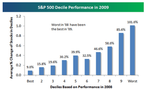
Pure contrarian investing is investing relying solely on the phenomenon of reversion to the mean without making an assessment of value. Is it possible to observe the effects of mean reversion by constructing a portfolio on a basis other than some indicia of value? It is, and the Bespoke Investment Group has done all the heavy lifting for us. Bespoke constructed from the S&P500 ten portfolios with 50 stocks in each on the basis of stock performance in 2008. They then tracked the performance of those stocks in 2009. The result?

Many of the stocks that got hit the hardest last year came roaring back this year, and the numbers below help quantify this.  As shown, the 50 stocks in the S&P 500 that did the worst in 2008 are up an average of 101% in 2009!  The 50 stocks that did the best in 2008 are up an average of just 9% in 2009.  2009 was definitely a year when buying the losers worked.

It’s a stunning outcome, and it seems that the portfolios (almost) performed in rank order. While there may be a value effect in these results, the deciles were constructed on price performance alone. This would seem to indicate that, at an aggregate level at least, mean reversion is a powerful phenomenon and a pure contrarian investment strategy relying on mean reversion should work.

Read Full Post »

In his 2006 research report Painting By Numbers: An Ode To Quant (via The Hedge Fund Journal) James Montier presents a compelling argument for a quantitative approach to investing. Montier’s thesis is that simple statistical or quantitative models consistently outperform expert judgements. This phenomenon continues even when the experts are provided with the models’ predictions. Montier argues that the models outperform because humans are overconfident, biased, and unable or unwilling to change.

Montier makes his argument via a series of examples drawn from fields other than investment. The first example he gives, which he describes as a “classic in the field” and which succinctly demonstrates the two important elements of his thesis, is the diagnosis of patients as either neurotic or psychotic. The distinction is as follows: a psychotic patient “has lost touch with the external world” whereas a neurotic patient “is in touch with the external world but suffering from internal emotional distress, which may be immobilising.” According to Montier, the standard test to distinguish between neurosis or psychosis is the Minnesota Multiphasic Personality Inventory or MMPI:

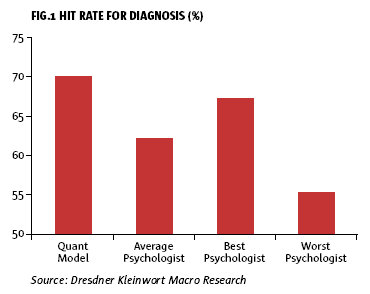
In 1968, Lewis Goldberg1 obtained access to more than 1000 patients’ MMPI test responses and final diagnoses as neurotic or psychotic. He developed a simple statistical formula, based on 10 MMPI scores, to predict the final diagnosis. His model was roughly 70% accurate when applied out of sample. Goldberg then gave MMPI scores to experienced and inexperienced clinical psychologists and asked them to diagnose the patient. As Fig.1 shows, the simple quant rule significantly outperformed even the best of the psychologists.

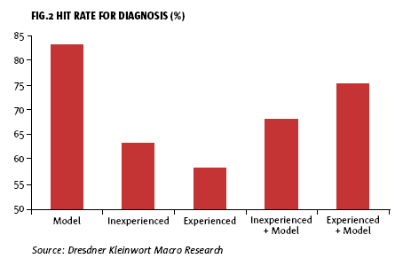
Even when the results of the rules’ predictions were made available to the psychologists, they still underperformed the model. This is a very important point: much as we all like to think we can add something to the quant model output, the truth is that very often quant models represent a ceiling in performance (from which we detract) rather than a floor (to which we can add).

The MMPI example illustrates the two important points of Montier’s thesis:

  1. The simple statistical model outperforms the judgements of the best experts.
  2. The simple statistical model outperforms the judgements of the best experts, even when those experts are given access to the simple statistical model.

Montier goes on to give diverse examples of the application of his theory, ranging from the detection of brain damage, the interview process to admit students to university, the likelihood of a criminal to re-offend, the selection of “good” and “bad” vintages of Bordeaux wine, and the buying decisions of purchasing managers. He then discusses some “meta-analysis” of studies to demonstrate that “the range of evidence I’ve presented here is not somehow a biased selection designed to prove my point:”

Grove et al consider an impressive 136 studies of simple quant models versus human judgements. The range of studies covered areas as diverse as criminal recidivism to occupational choice, diagnosis of heart attacks to academic performance. Across these studies 64 clearly favoured the model, 64 showed approximately the same result between the model and human judgement, and a mere 8 studies found in favour of human judgements. All of these eight shared one trait in common; the humans had more information than the quant models. If the quant models had the same information it is highly likely they would have outperformed.

As Paul Meehl (one of the founding fathers of the importance of quant models versus human judgements) wrote: There is no controversy in social science which shows such a large body of qualitatively diverse studies coming out so uniformly in the same direction as this one… predicting everything from the outcomes of football games to the diagnosis of liver disease and when you can hardly come up with a half a dozen studies showing even a weak tendencyin favour of the clinician, it is time to draw a practical conclusion.

Why not investing?

Montier says that, within the world of investing, the quantitative approach is “far from common,” and, where it does exist, the practitioners tend to be “rocket scientist uber-geeks,” the implication being that they would not employ a simple model. So why isn’t quantitative investing more common? According to Montier, the “most likely answer is overconfidence.”

We all think that we know better than simple models. The key to the quant model’s performance is that it has a known error rate while our error rates are unknown.

The most common response to these findings is to argue that surely a fund manager should be able to use quant as an input, with the flexibility to override the model when required. However, as mentioned above, the evidence suggests that quant models tend to act as a ceiling rather than a floor for our behaviour. Additionally there is plenty of evidence to suggest that we tend to overweight our own opinions and experiences against statistical evidence.

Montier provides the following example is support of his contention that we tend to prefer our own views to statistical evidence:

For instance, Yaniv and Kleinberger11 have a clever experiment based on general knowledge questions such as: In which year were the Dead Sea scrolls discovered?

Participants are asked to give a point estimate and a 95% confidence interval. Having done this they are then presented with an advisor’s suggested answer, and asked for their final best estimate and rate of estimates. Fig.7 shows the average mean absolute error in years for the original answer and the final answer. The final answer is more accurate than the initial guess.

The most logical way of combining your view with that of the advisor is to give equal weight to each answer. However, participants were not doing this (they would have been even more accurate if they had done so). Instead they were putting a 71% weight on their own answer. In over half the trials the weight on their own view was actually 90-100%! This represents egocentric discounting – the weighing of one’s own opinions as much more important than another’s view.

Similarly, Simonsohn et al12 showed that in a series of experiments direct experience is frequently much more heavily weighted than general experience, even if the information is equally relevant and objective. They note, “If people use their direct experience to assess the likelihood of events, they are likely to overweight the importance of unlikely events that have occurred to them, and to underestimate the importance of those that have not”. In fact, in one of their experiments, Simonsohn et al found that personal experience was weighted twice as heavily as vicarious experience! This is an uncannily close estimate to that obtained by Yaniv and Kleinberger in an entirely different setting.

It is worth noting that Montier identifies LSV Asset Management and Fuller & Thaler Asset Management as being “fairly normal” quantitative funds (as opposed to being “rocket scientist uber-geeks”) with “admirable track records in terms of outperformance.” You might recognize the names: “LSV” stands for Lakonishok, Shleifer, and Vishny, authors of the landmark Contrarian Investment, Extrapolation and Risk paper, and the “Thaler” in Fuller & Thaler is Richard H. Thaler, co-author of Further Evidence on Investor Overreaction and Stock Market Seasonality, both papers I’m wont to cite. I’m not entirely sure what strategies LSV and Fuller & Thaler pursue, wrapped as they are in the cloaks of “behavioural finance,” but judging from those two papers, I’d say it’s a fair bet that they are both pursuing value-based strategies.

It might be a while before we see a purely quantitative value fund, or at least a fund that acknowledges that it is one. As Montier notes:

We find it ‘easy’ to understand the idea of analysts searching for value, and fund managers rooting out hidden opportunities. However, selling a quant model will be much harder. The term ‘black box’ will be bandied around in a highly pejorative way. Consultants may question why they are employing you at all, if ‘all’ you do is turn up and run the model and then walk away again.

It is for reasons like these that quant investing is likely to remain a fringe activity, no matter how successful it may be.

Montier’s now at GMO, and has produced a new research report called Ten Lessons (Not?) Learnt (via Trader’s Narrative).

Read Full Post »

The Wall Street Journal’s Deal Journal blog has an article, The Secret to M&A: It Pays to Be Humble, about a KPMG study into the factors determining the success or otherwise of M&A deals over the period from 2002 to 2006. Some of the results are a little unexpected. Most surprising: acquirers purchasing targets with higher P/E ratios outperformed acquirers of targets with lower P/E ratios, which seems to fly in the face of every study I’ve ever read, and calls into question everything that is good and holy in the world. In effect, KPMG is saying that the relationship of value as a predictor of investment returns broke down for the period studied. I think it’s an aberration, and I’ll be sticking with value as my strategy.

In the study, The Determinants of M&A Success What Factors Contribute to Deal Success? (.pdf), KPMG examined a number of variables to determine which had a statistically significant influence on the stock performance of the acquirer. Those variables examined included the following:

  • How the deal was financed—stock vs. cash, or both
  • The size of the acquirer
  • The price-to-earnings (“P/E”) ratio of the acquirer
  • The P/E ratio of the target
  • The prior deal experience of the acquirer
  • The stated deal rationale
  • Whether or not the deal was cross-border

KPMG found that some factors were highly correlated with success (for example, paying with cash, rather than using stock or cash and stock) and others were not statistically significant (surprisingly, market capitalization). Here are KPMG’s “key findings”:

  • Cash-only deals had higher returns than stock-and-cash deals, and stock-only deals
  • Acquirers with low price-to-earnings (P/E) ratios resulted in more successful deals
  • Those companies that closed three to five deals were the most successful; closing more than five deals in a year reduced success
  • Transactions that were motivated by increasing “financial strength” were most successful
  • The size of the acquirer (based on market capitalization) was not statistically significant

The P/E ratio of the target is correlated with success, but not in the manner that one might expect:

The P/E ratio of the target was also statistically significant. In contrast to our previous study, acquirers who were able to purchase companies with P/E ratios below the industry median saw a negative 6.3 percent return after one year and a negative 6.0 percent return after two years. Acquirers who purchased targets with P/E ratios above the median, including those with negative P/E ratios, had a negative 1 percent return after one year and a negative 3.5 percent return after two years. These results are very different from the ones we found in our last study for deals announced between 2000 and 2004. Those earlier deals demonstrated the more anticipated results: acquirers who purchased targets with below average P/E ratios were more successful than acquirers who purchased targets with higher P/E ratios.

It is probable that in the deals announced between 2002 and 2006, acquirers who purchased targets with high P/E ratios were buying businesses that were growing and where the acquirer was able to achieve greater synergies. Deals announced between 2000 and 2004 included deals from the “dot-com” era, where high P/E ratios were often associated with unprofitable ventures that were not able to meet future income expectations.

Here’s the chart showing the relative returns to P/E:

Now, we value folk know that, in any given instance, the P/E ratio alone tells us little about the sagacity of an investment. In the aggregate, however, we would have expected the lower P/E targets to outperform the more expensive acquisitions. That’s not just wishful thinking, it’s based on the various studies that I am so fond of quoting, most notably Lakonishok, Shleifer, and Vishny’s Contrarian Investment, Extrapolation and Risk. Lakonishok, Shleifer, and Vishny found that “value”determined on the basis of P/E consistently outperformed “glamour”. That relationship seems to have broken down over the period 2002 to 2006 according to the KPMG study.

There are several possible explanations for KPMG’s odd finding. First, they weren’t directly tracking the performance of the stock of the target, they were analysing the performance of the stock of the acquirer, which means that other factors in the acquirers’ stocks could have influenced the outcome. Second, five years is a relatively short period to study. A longer study may have resulted in the usual findings. Third, it’s possible that 2002 to 2006 was a period where the traditional value phenomenon broke down. It was a big leg up in the market, and a bull market makes everyone look like a genius. Perhaps it didn’t matter what an acquirer paid. That seems unlikely, because the stocks of the acquirers were generally down over the period. Finally, KPMG might have taken an odd sample. They looked at acquisitions “where acquirers purchased 100 percent of the target, where the target constituted at least 20 percent of the sales of the acquirer and where the purchase price was in excess of US$100 million. The average deal size of the transactions in this study was US$3.4 billion; the median was US$0.7 billion.” Perhaps that slice of the market is different from the rest of the market. Again, that seems unlikely. I think KPMG’s finding is an aberration. I certainly wouldn’t turn it into a strategy.

Read Full Post »

« Newer Posts - Older Posts »