Greenbackd

I received a number of emails asking me to revisit the backtests from last week’s post about using the Shiller PE to time the market (Worried about a Crash? Backtests Using Shiller PE to Time The Market (1926 to 2014)). The most common request was to separate the buy and sell rules such that if the strategy sold out at say one standard deviation above the mean, it didn’t buy back until the Shiller PE fell below its mean. The second most common request was to alter the strategy such that it hedged out the market rather than switching to cash.

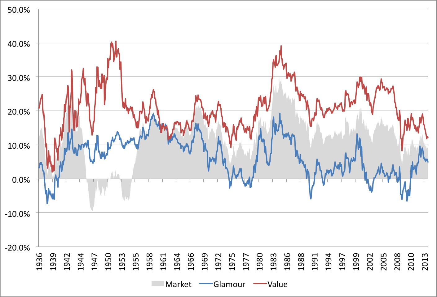
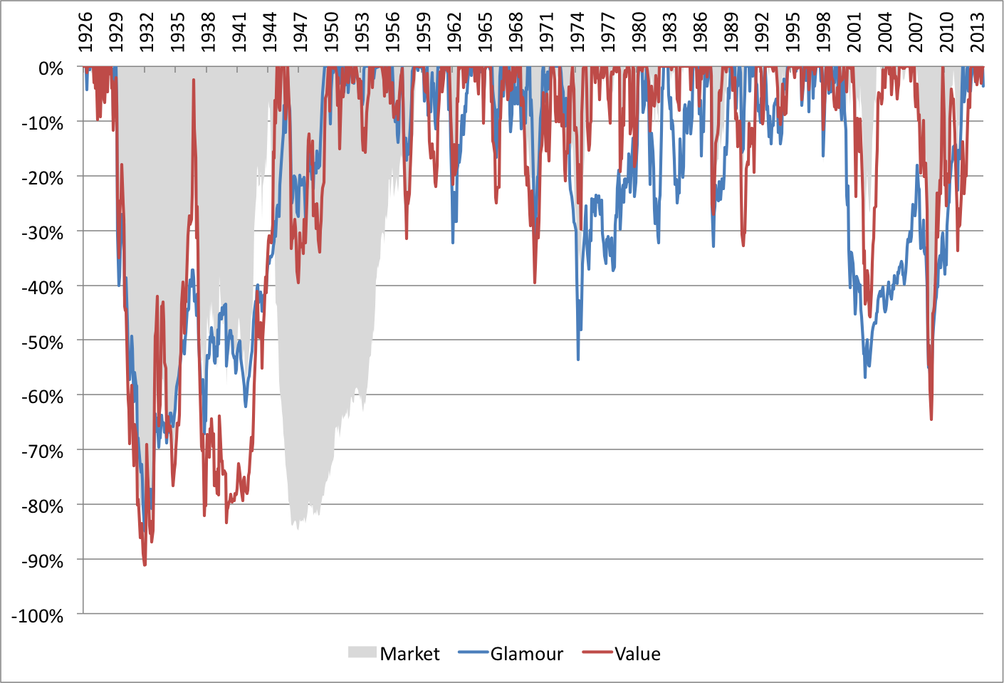
Edit: Fama and French backtests of the book value-to-market equity (the inverse of the PB ratio) data from 1926 to 2013. As at December 2013, there were 3,175 firms in the sample. The value decile contained the 459 stocks with the highest earnings yield, and the glamour decile contained the 404 stocks with the lowest earnings yield. The average size of the glamour stocks is $7.48 billion and the value stocks $2.54 billion. (Note that the average is heavily skewed up by the biggest companies. For context, the 3,175th company has a market capitalization today of $404 million, which is smaller than the average, but still investable for most investors). Portfolios are formed on June 30 and rebalanced annually.

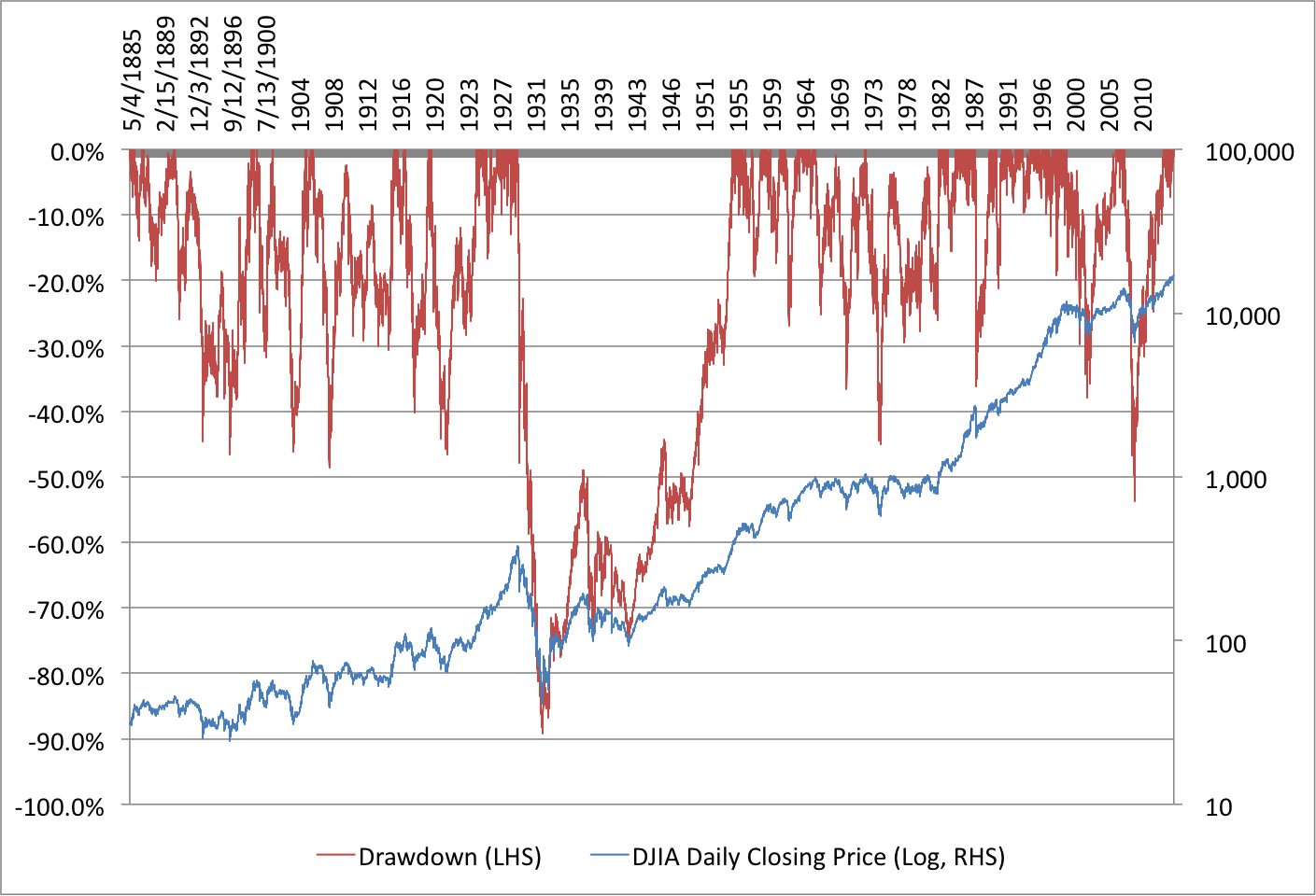
The following backtests use the market’s state of knowledge at the time about the average, and standard deviations of the Shiller PE. The chart below shows how the Shiller PE’s average and standard deviations have varied over time.

Shiller PE, Average, and Plus/Minus Two Standard Deviations (1881 to Present)

The mean now is 16.55, but was as low as 14.2 in the 1950s and, excluding the slightly higher reading at the start of the data, as high as 17.5 in the 1900s. The standard deviation has expanded over time. Until the 2000s two standard deviations above the average meant a Shiller PE of about 25, and now it means a Shiller PE of almost 30.

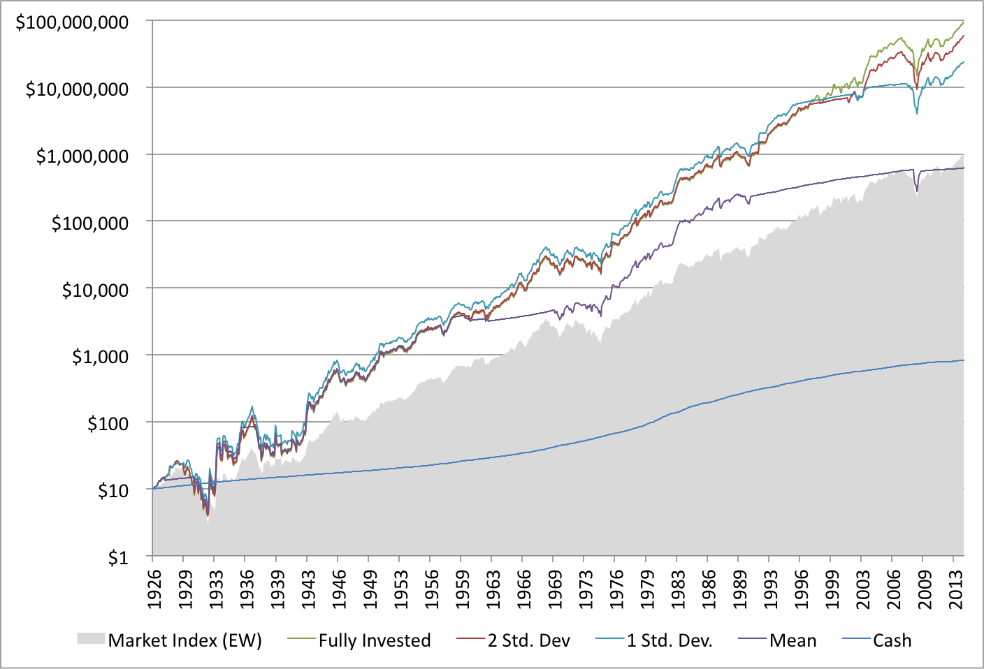
Performance of Value Decile (Price-to-Book Value), Cash and 3 Shiller PE Timed Strategies (1926 to Present)

The following chart backtests three strategies. The first–“Sell at 1SD, Buy at -1SD”–buys the price-to-book value decile only if the Shiller PE is one standard deviation below its mean, sells into cash if the Shiller PE is more than one standard deviation above its mean, and holds cash until the market falls back below one standard deviation below the mean. The second–“Sell at 1SD, Buy at Mean”–buys the price-to-book value decile only if the Shiller PE is below its mean, sells into cash if the Shiller PE is more than one standard deviation above its mean, and holds cash until the market falls back below the mean. The third–“Sell at 2SD, Buy at Mean”–buys the value decile only if the Shiller PE is below its mean, sells into cash if the Shiller PE is more than two standard deviations above its mean, and holds cash until the market falls back below the mean.

All the strategies underperform the simple buy-and-hold strategy over the full period.

The market returned 13.94 percent compound and the fully invested PB value decile returned 20 percent compound over the full period. Sell at 1SD, Buy at -1SD returned 15.0 percent compound; Sell at 2SD, Buy at Mean returned 19.3 percent compound; and Sell at 1SD, Buy at Mean returned 15.9 percent compound.

Sell at 2SD, Buy at Mean had good lead until the 1990s, but has woefully underperformed since. Notably, it is still fully invested. Its sell rule won’t kick in until the Shiller PE hits 29.7.

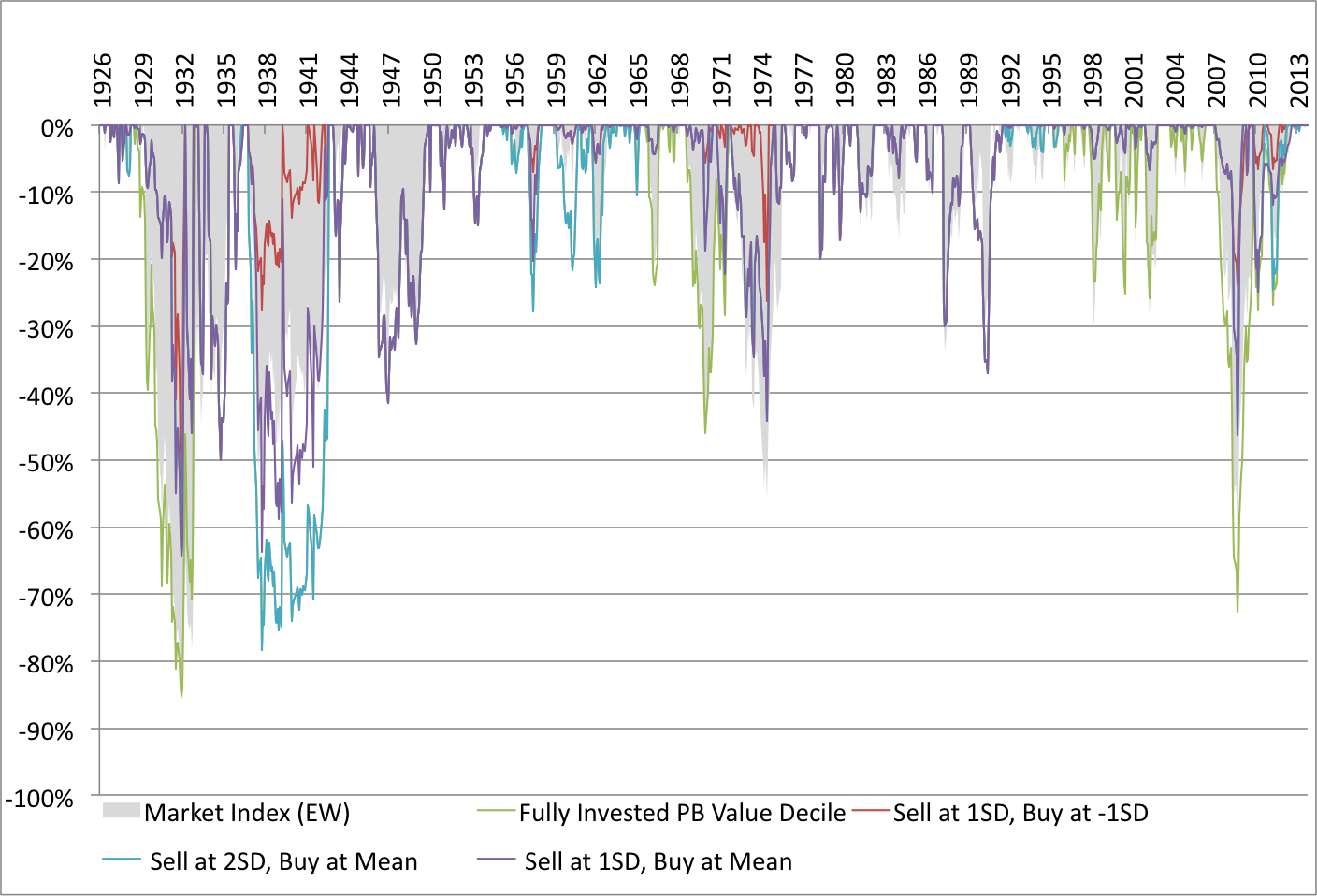
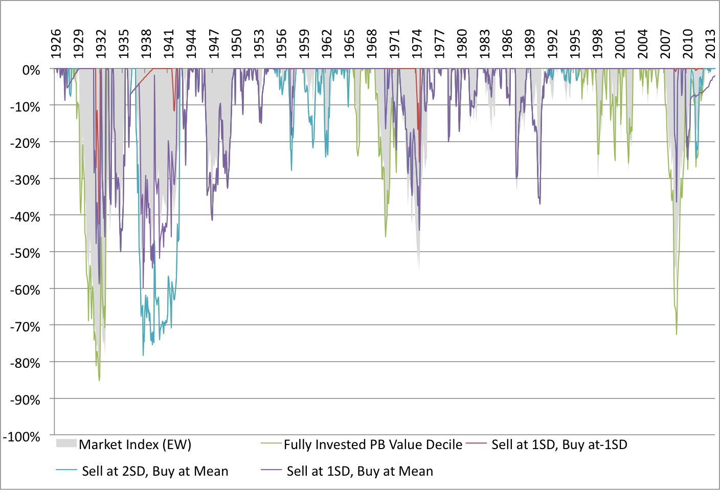
Drawdowns of Value Decile (Price-to-Book Value), Cash and 3 Shiller PE Timed Strategies (1926 to Present)

The market has the worst maximum drawdown at 86 percent, and the fully invested PB value decile has a comparably bad maximum drawdown of 85 percent. Sell at 1SD, Buy at -1SD had the best maximum drawdown at 50 percent; Sell at 2SD, Buy at Mean had a maximum drawdown of 78 percent; and Sell at 1SD, Buy at Mean had a maximum drawdown of 60 percent.

Graham Rule: Performance of Value Decile (Price-to-Book Value), Cash and 3 Shiller PE Timed Strategies (1926 to Present)

Benjamin Graham recommended maintaining a minimum portfolio exposure to stocks of 25 percent. Below we re-run the tests, but this time instead of kicking all of the portfolio into cash, we put only 75 of the portfolio in cash, and maintain 25 percent exposure to the value decile.

All the returns are improved, but the strategies continue to underperform the simple buy-and-hold strategy over the full period.

Sell at 1SD, Buy at -1SD now returns 16.8 percent compound; Sell at 2SD, Buy at Mean returned 19.6 percent compound versus 19.3 percent above; and Sell at 1SD, Buy at Mean returned 17.2 percent compound.

Graham Rule: Drawdowns of Value Decile (Price-to-Book Value), Cash and 3 Shiller PE Timed Strategies (1926 to Present)

The tradeoff for slightly improved returns is slightly worse drawdowns. Sell at 1SD, Buy at -1SD still has the lowest maximum drawdown, but now draws down 53 percent; Sell at 2SD, Buy at Mean has the same maximum drawdown of 78 percent; and Sell at 1SD, Buy at Mean had a maximum drawdown of 64 percent.

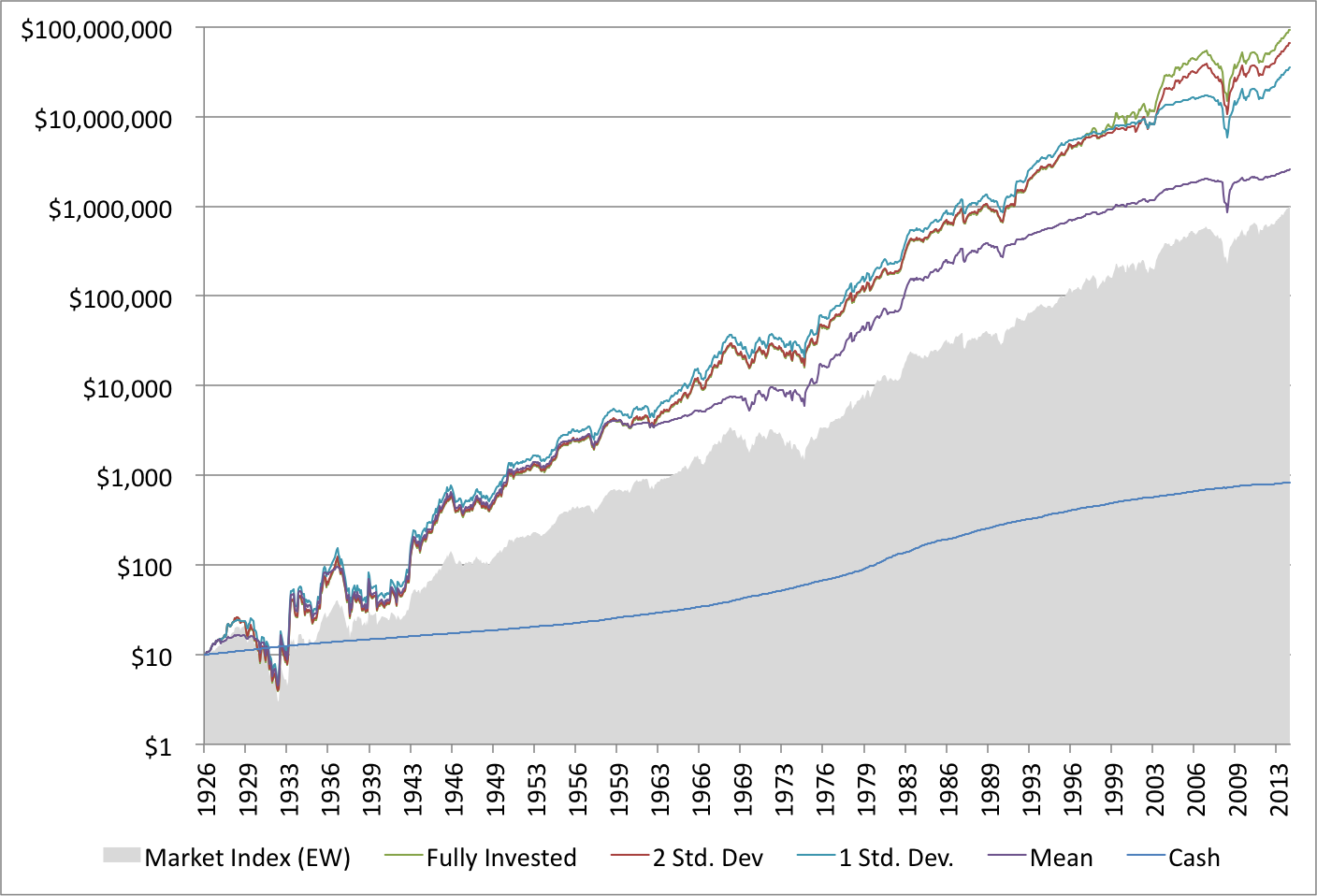
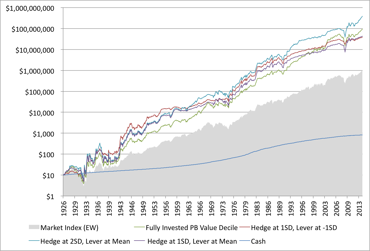
Market Hedge: Performance of Value Decile (Price-to-Book Value), Cash and 3 Shiller PE Timed Strategies (1926 to Present)

In this set of backtests the strategy is levered and hedged. The ratios change depending on the level of the market. When the strategy deems the market cheap, it is 130 percent long the value decile, and 30 short the market. When the market is expensive, it doesn’t sell into cash, but reduces the long to 100 percent, and hedges out 75 percent of the portfolio using the market.

The Hedge at 2SD, Lever at Mean strategy outperforms the buy-and-hold strategy over the full period, returning 21.9 percent compound, versus 20 percent for the value decile.

Hedge at 1SD, Lever at -1SD now returns 19 percent compound; and Hedge at 1SD, Buy at Mean returned 18.9 percent compound.

Market Hedge: Drawdowns of Value Decile (Price-to-Book Value), Cash and 3 Shiller PE Timed Strategies (1926 to Present)

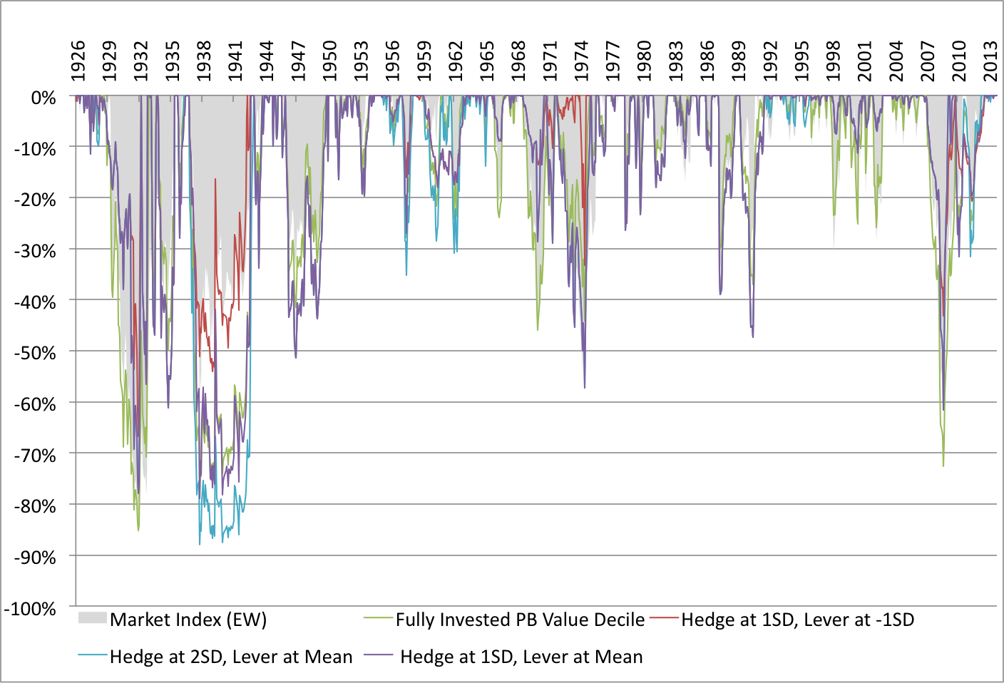
The tradeoff for the improved returns is bigger drawdowns.

Hedge at 2SD, Lever at Mean strategy draws down 88 percent, worse than the market’s 85 percent; Hedge at 1SD, Lever at -1SD has a maximum draw down of 67 percent; and Hedge at 1SD, Buy at Mean has a maximum drawdown of 79 percent.

Changing the buy-and-sell rules, and hedging rather than running to cash alters the performance of the strategies. The levered and hedged strategy that maximizes exposure to the market–Hedge at 2SD, Lever at Mean–outperforms the simple buy-and-hold strategy, but does so with an enormous drawdown. Nothing else beats buy-and-hold. As we saw last week, the more conservative the Shiller PE ratio used, the lower the drawdown, but returns suffer. To generate the extraordinary returns of the value deciles I’ve examined over the last few weeks, it was necessary to remain fully invested in those value stocks through thick and thin. My firm, Eyquem, offers low cost, fee-only managed accounts that implement a systematic deep value investment strategy. Please contact me by email at toby@eyquem.net or call me by telephone on (646) 535 8629 to learn more. Click here if you’d like to read more on Quantitative Value, or connect with me on Twitter, LinkedIn or Facebook.

Read Full Post »

Charlie and I would much rather earn a lumpy 15% over time than a smooth 12%.

–Buffett, Chairman’s Letter (1996)

Can an investor concerned about a big crash use a systematic timing tool to exit the market before the crash without giving up too much return? One possible method for doing so is to use the Shiller PE as a valuation tool, and to move the portfolio into cash at some given level of overvaluation. The backtests below show the returns and drawdowns for exiting at four different levels of the Shiller PE ratio, from aggressive to conservative.

The first option is to simply always remain fully invested in the value decile (measured by price-to-book value). For our present purposes, this is the most aggressive. The three other timed strategies kick out of the value decile when the Shiller PE gets increasingly expensive. Mean, the most conservative kicks into cash when the Shiller PE gets just above its mean (17.6 for the data set). Slightly more aggressive is a strategy that kicks into cash at one standard deviation above the mean (a Shiller PE of 24.8) called 1 Std. Dev., and the next most aggressive kicks out at two standard deviations above the long-run average (a Shiller PE of 32.0) called 2 Std. Dev..

Edit: The backtests use Fama and French backtests of the book value-to-market equity (the inverse of the PB ratio) data from 1926 to 2013. As at December 2013, there were 3,175 firms in the sample. The value decile contained the 459 stocks with the highest earnings yield, and the glamour decile contained the 404 stocks with the lowest earnings yield. The average size of the glamour stocks is $7.48 billion and the value stocks $2.54 billion. (Note that the average is heavily skewed up by the biggest companies. For context, the 3,175th company has a market capitalization today of $404 million, which is smaller than the average, but still investable for most investors). Portfolios are formed on June 30 and rebalanced annually.

Performance of Value Decile (Price-to-Book Value), Cash and 3 Shiller PE Timed Strategies

Over the period examined, the market (the equally weighted universe from which the portfolios were drawn) generated a compound average growth rate (CAGR) of 13.94 percent. Cash generated an average return of 5.17 percent over the same period. The fully invested value decile generated the best CAGR over the full period at 20.01 percent. The other strategies underperformed to the extent that they remained out of the market: The strategy that kicked into cash at the mean returned 13.4 percent yearly, the strategy that kicked into cash at one standard deviation above the mean returned 18.15 percent yearly, and the strategy that kicked into cash at two standard deviations above the mean returned 19.36 percent compound over the full period.

We expect underperformance for remaining out of the market. This is the tradeoff we make to avoid drawdowns. Is it worth it? Below we examine how much drawdown we avoid by getting out of the market at the different ratios.

Drawdowns to Value Decile (Price-to-Book Value), and 3 Shiller PE Timed Strategies

The market had a maximum drawdown in 1929 of 86 percent, and has a Sharpe ratio over the full period of of 0.13. The fully invested strategy had a maximum drawdown of 85 percent, and generated a Sharpe ratio of 0.15. The other strategies generate lower maximum drawdowns, but do so for lower Sharpe ratios: The strategy that kicked into cash at the mean had a maximum drawdown of 69 percent, and the worst Sharpe ratio at 0.11;  the strategy that kicked into cash at one standard deviation above the mean had a maximum drawdown of 80 percent, and a Sharpe ratio of 0.14, and the strategy that kicked into cash at two standard deviations above the mean had a maximum drawdown of 84 percent, and a Sharpe ratio of 0.15.

Drawdowns Relative to the Market for Value Decile (Price-to-Book Value), and 3 Shiller PE Timed Strategies

This chart examines the drawdown to each strategy relative to the market. Where it is below the midline, the strategy has drawn down further than the market, and above the midline it is outperforming.

Benjamin Graham recommended maintaining a minimum portfolio exposure to stocks of 25 percent. Below we re-run the tests, but this time instead of kicking all of the portfolio into cash, we put only 75 of the portfolio in cash, and maintain 25 percent exposure to the value decile.

Performance of Value Decile (Price-to-Book Value), Cash and 3 Shiller PE Timed Strategies (Graham Rule)

The additional exposure to the market improves the returns for the three timed strategies. The strategy that kicked into cash at the mean now returns 15.23 percent yearly, the strategy that kicked into cash at one standard deviation above the mean returned 18.67 percent yearly, and the strategy that kicked into cash at two standard deviations above the mean returned 19.55 percent compound over the full period. All still underperform the fully invested strategy at 20.01 percent.

Drawdowns to Value Decile (Price-to-Book Value), Cash and 3 Shiller PE Timed Strategies

The tradeoff for slightly improved returns is greater drawdowns and volatility. The strategy that kicked into cash at the mean had lower a maximum drawdown of 73 percent, but an improved Sharpe ratio at 0.12;  the strategy that kicked into cash at one standard deviation above the mean remained unchanged with a maximum drawdown of 80 percent, and a Sharpe ratio of 0.14, and the strategy that kicked into cash at two standard deviations above the mean had a maximum drawdown of 85 percent, and a Sharpe ratio of 0.15.

Drawdowns Relative to the Market for Value Decile (Price-to-Book Value), and 3 Shiller PE Timed Strategies

The Shiller PE is not a particularly useful timing mechanism. This is because valuation is not good at timing the market (really, nothing works–timing the market is a fool’s or genius’s game). Carrying cash does serve to reduce drawdowns. It also reduces returns. The more conservative the Shiller PE ratio used, the lower the drawdown, but returns suffer, and Sharpe ratios reduce. To generate the extraordinary returns of the value deciles I’ve examined over the last few weeks, it was necessary to remain fully invested in those value stocks through thick and thin. My firm, Eyquem, offers low cost, fee-only managed accounts that implement a systematic deep value investment strategy. Please contact me by email at toby@eyquem.net or call me by telephone on (646) 535 8629 to learn more. Click here if you’d like to read more on Quantitative Value, or connect with me on Twitter, LinkedIn or Facebook.

Read Full Post »

The 10^th Annual New York Value Investing Congress is just weeks away (Sept. 8-9), ​but there’s still time to ​get your seat and enjoy the many benefits of attending the Congress in-person:

• Speaker ​Wisdom – Congress speakers explain their stock ideas with detailed, well-reasoned analysis.  But the presentations are not live-streamed or distributed afterwards,so only onsite attendees benefit from the ​brilliance of these ​successful money managers.

• Audience Q&A – Congress attendees are savvy, professional investors and their insightful questions often clarify and expand on a speaker’s investment thesis.  As with speaker commentary, live Q&A is only available to onsite attendees.

• Exclusive Information – The Congress is closed to the media and live bloggers– our attendees benefit first from actionable information.

• Great Networking –  The VIC Cocktail Reception has become a favorite among attendees for sharing new ideas, creating new business opportunities and making friendships that ​can last a lifetime.

Register now and benefit from attending the Congress in-person.  But seats are strictly limited to 275, so we encourage Greenbackd readers to register now, before we sell out.

For a special Greenbackd Discount, register now with Offer Code: GREENBACKD  at Valueinvestingcongress.com/congress/register-now-partners/

Confirmed Speakers include:

• Leon Cooperman, Omega Advisors
• Sahm Adrangi, Kerrisdale Capital Management
• Carson Block, Muddy Waters Research
• Andrew Left, Citron Research
• Alexander Roepers, Atlantic Investment Management
• Jeffrey Smith, Starboard Value
• Amitabh Singhi, Surefin Investments
• Guy Spier, Aquamarine Fund
• David Hurwitz, SC Fundamental
• Michael Kao, Akanthos Capital
• Guy Gottfried, Rational Capital Management
• Adam Crocker, Metropolitan Capital Advisors
• Whitney Tilson, Kase Capital
• John Lewis, Osmium Partners
• Tim Eriksen, Eriksen Capital Management
• Cliff Remily, Northwest Priority Capital
• With more to come!

Read Full Post »

I’ve been digging back through some very old historical data to understand how unusual the 1929 crash was and found the site Measuring Worth, which has the interesting mission “to make available to the public the highest quality and most reliable historical data on important economic aggregates.” Measuring Worth has a data series combining the Dow Jones Industrial Average and its precursor, the Dow Jones Average, all the way back to May 1885. Measuring Worth provides this fascinating history of the index:

On July 3, 1884, Charles Henry Dow began publishing his Dow Jones Average. By the time it was published daily eight months later, the index was composed of 12 stocks, 10 of which were railroads. This index appeared in the Customer’s Afternoon Letter up until July 8, 1889 when the first issue of The Wall Street Journal was published. On October 7, 1896, Dow started publishing two “Daily Moving Averages,” 12 industrials and 20 railroads (that would later become the transportation index.) This first Dow Jones Industrial Average (DJIA) was published through September 29, 1916. This first DJIA closed at 71.42 on July 30, 1914 and so did the New York Stock Market for the next four months. Some historians believe the reason for this was worry that markets would plunge because of panic over the onset of the World War. An interesting book by William L. Silber titled When Washington Shut down Wall Street: The Great Financial Crisis of 1914 and the Origins of America’s Monetary Supremacy (2007) has a different explanation. He thinks that Secretary of the Treasury, William McAdoo closed the exchange because he wanted to conserve the US gold stock in order to launch the Federal Reserve System later that year with enough gold to keep the US on the gold standard. Whatever the reason, the first day it reopened on December 12, 1914, the index closed at 74.56, thus the War had not had the predicted impact. On October 4, 1916, the WSJ starts publishing a (new) DJIA of 20 stocks, 8 stocks from the old index and 12 new stocks. It was traced the index back to December 12, 1914 at that time. It is important to know that data for the first DJIA of 12 stocks and the second DJIA of 20 stocks are BOTH available for the 21 months and the first index was about 36% higher than the second and the data here are adjusted to make them a consistent time series. On October 1, 1928 the DJIA of 30 stocks was first quoted in the WSJ. It contained 14 stocks from the second list of 20 and 16 new stocks. Its level was consistent with the second list, so no adjustment was necessary.

In the chart below I’ve plotted the daily closing price for the series from May 1885 to Friday’s close (the blue line, log, right-hand side), along with the drawdowns (the red line, left-hand side).

Source: Samuel H. Williamson, ‘Daily Closing Value of the Dow Jones Average, 1885 to Present,’ MeasuringWorth, 2012.

For me there are two striking features on the chart. First, the 1929 crash is on a different scale to any other crash, dwarfing even the second biggest crash, which was the most recent one beginning in 2007. The 1929 crash began on September 4, 1929, and bottomed on July 8, 1932, down 89.2 percent. The market wouldn’t achieve its 1929 high again until November 23, 1954, more than 25 years from its last peak, and more than 22 years from the bottom. By way of contrast, the second deepest drawdown at -53.8 percent, the 2007 Credit Crisis began October 1, 2007, and ended March 4, 2013, a mere 5 years and 5 months later. The second longest drawdown began November 1905, bottomed down -48.5 percent, and ended almost 10 years later in July 1915.

The second striking feature of the chart is how much time the market spends in a drawdown. The market hits a new high about 3.8 percent of days, which means it’s in drawdown 96.2 percent of the time. In addition to the 1905 and 1929 crashes, there have been two other busts that lasted longer than 8 years, including one that ran from May 1890 and ended almost 9 years later in January 1899, and another that began January 1973, and ended November 2, 1982. And there were six more that lasted longer than four years. It makes me think we really should break out the Dow X,000 hats every time the market crosses a round number that’s a new all-time high.

It’s not all bad news. Since 1885, the Dow Jones is up 552 times, which equates to a compound annual growth rate of about 5 percent (this excludes the impact of dividends, which have been material, to the tune of around 4 percent more on average, and 1.9 percent today). From the 1932 bottom to the next all-time high in November 1954, the market returned more than double that rate at 10.6 percent. Drawdowns are the usual condition of investing, but, over the very long term, the market has continued to grow. To generate the extraordinary returns of the value deciles I’ve examined over the last few weeks, it was necessary to remain fully invested in those value stocks through thick and thin. My firm, Eyquem, offers low cost, fee-only managed accounts that implement a systematic deep value investment strategy. Please contact me by email at toby@eyquem.net or call me by telephone on (646) 535 8629 to learn more. Click here if you’d like to read more on Quantitative Value, or connect with me on LinkedIn.

Read Full Post »

I’ve been reading John F. Wasik’s Keynes’s Way to Wealth: Timeless Investment Lessons from The Great Economist, a book about British economist John Maynard Keynes’s life as an investor. Keynes started out as a foreign currency and commodity speculator in 1919, was wiped out twice in 1922, and 1929, and went on to become a Buffett-style concentrated value investor by around 1932. In 1991, Buffett, who noted in an earlier Chairman’s letter that Keynes had “began as a market-timer (leaning on business and credit-cycle theory) and converted, after much thought, to value investing,” described Keynes’s end-point as an investor thus:

John Maynard Keynes, whose brilliance as a practicing investor matched his brilliance in thought, wrote a letter to a business associate, F. C. Scott, on August 15, 1934 that says it all: “As time goes on, I get more and more convinced that the right method in investment is to put fairly large sums into enterprises which one thinks one knows something about and in the management of which one thoroughly believes. It is a mistake to think that one limits one’s risk by spreading too much between enterprises about which one knows little and has no reason for special confidence. . . .

One’s knowledge and experience are definitely limited and there are seldom more than two or three enterprises at any given time in which I personally feel myself entitled to put full confidence.”

Wasik reports that Keynes died in 1946 with a net worth of about £500,000, equivalent to about $36 million today, not including his extensive collection of artwork and rare manuscripts.

What is most remarkable about Keynes is that he was a self-taught Buffett-style concentrated value investor before Buffett. He wrote the letter to Scott around the time that Benjamin Graham published Security Analysis, but there is little evidence that he read it. Like Graham, Keynes had to contend with perhaps the most difficult period in modern history to be an investor, one that encompassed the second World War, the 1929 stock market crash, and the Great Depression. Throughout that 18-year period, while the UK stock market fell 15 percent, and the US market fell 21 percent, the discretionary portfolio he managed on behalf of King’s College, Cambridge grew fivefold.

The charts below, which begin in 1926 and continue through to April 2014, show how unusually difficult the period was. The charts use Fama and French backtests of the book value-to-market equity (the inverse of the PB ratio) data from 1926 to 2014. As at April 2014, there were 3,175 firms in the sample. The value decile contained the 459 stocks with the highest earnings yield, and the glamour decile contained the 404 stocks with the lowest earnings yield. The average size of the glamour stocks is $7.48 billion and the value stocks $2.54 billion. (Note that the average is heavily skewed up by the biggest companies. For context, the 3,175th company has a market capitalization today of approximately $400 million, which is smaller than the average, but still investable for most investors). Portfolios are formed on June 30 and rebalanced annually.

Compound Returns 1926 to April 2014 (Market Capitalization Weight)

The 1938 crash also hit Keynes hard. At the end of the year, his King’s College discretionary portfolio was down 40.1 percent.

10-Year Rolling Returns (Market Capitalization Weight)

Drawdowns (Market Capitalization Weight)

Compound Returns 1926 to April 2014 (Equal Weight)

10-Year Rolling Returns (Equal Weight)

Drawdowns (Equal Weight)

As these charts demonstrate, volatility and drawdowns are part and parcel of investing, but, over the long term, value has comprehensively beaten out the market and glamour stocks. To generate the extraordinary returns of the value deciles, it was necessary to remain fully invested in those value stocks through thick and thin. My firm, Eyquem, offers low cost, fee-only managed accounts that implement a systematic deep value investment strategy. Please contact me by email at toby@eyquem.net or call me by telephone on (646) 535 8629 to learn more.

Click here if you’d like to read more on Quantitative Value, or connect with me on LinkedIn.

Read Full Post »