Feeds:
Posts
Comments

Archive for the ‘Quantitative investment’ Category

I’ve just finished Ian Ayres’s book Super Crunchers, which I found via Andrew McAfee’s Harvard Business Review blog post, The Future of Decision Making: Less Intuition, More Evidence (discussed in Intuition and the quantitative value investor). Super Crunchers is a more full version of James Montier’s 2006 research report, Painting By Numbers: An Ode To Quant, providing several more anecdotes in support of Montier’s thesis that simple statistical models outperform the best judgements of experts. McAfee discusses one such example in his blog post:

Princeton economist Orley Ashenfleter predicts Bordeaux wine quality (and hence eventual price) using a model he developed that takes into account winter and harvest rainfall and growing season temperature. Massively influential wine critic Robert Parker has called Ashenfleter an “absolute total sham” and his approach “so absurd as to be laughable.” But as Ian Ayres recounts in his great book Supercrunchers, Ashenfelter was right and Parker wrong about the ‘86 vintage, and the way-out-on-a-limb predictions Ashenfelter made about the sublime quality of the ‘89 and ‘90 wines turned out to be spot on.

Ayers provides a number of stories not covered in Montier’s article, from Don Berwick’s “100,000 lives” campaign, Epagogix’s hit movie predictor, Offermatica’s automated web ad serving software, Continental Airlines’s complaint process, and a statistical algorithm for predicting the outcome of Supreme Court decisions. While seemingly unrelated, all are prediction engines based on a quantitative analysis of subjective or qualitative factors.

The Supreme Court decision prediction algorithm is particularly interesting to me, not because I am an ex-lawyer, but because the language of law is language, not often plain, and seemingly irreducible to quantitative analysis. (I believe this is true also of value investment, although numbers play a larger role in that realm, and therefore it lends itself more readily to quantitative analysis.) According to Andrew Martin and Kevin Quinn, the authors of Competing Approaches to Predicting Supreme Court Decision Making, if they are provided with just a few variables concerning the politics of a case, they can predict how the US Supreme Court justices will vote.

Ayers discussed the operation of Martin and Quinn’s Supreme Court decision prediction algorithm in How computers routed the experts:

Analysing historical data from 628 cases previously decided by the nine Supreme Court justices at the time, and taking into account six factors, including the circuit court of origin and the ideological direction of that lower court’s ruling, Martin and Quinn developed simple flowcharts that best predicted the votes of the individual justices. For example, they predicted that if a lower court decision was considered “liberal”, Justice Sandra Day O’Connor would vote to reverse it. If the decision was deemed “conservative”, on the other hand, and came from the 2nd, 3rd or Washington DC circuit courts or the Federal circuit, she would vote to affirm.

Ted Ruger, a law professor at the University of Pennsylvania, approached Martin and Quinn at a seminar and suggested that they test the performance of the algorithm against a group of legal experts:

As the men talked, they decided to run a horse race, to create “a friendly interdisciplinary competition” to compare the accuracy of two different ways to predict the outcome of Supreme Court cases. In one corner stood the predictions of the political scientists and their flow charts, and in the other, the opinions of 83 legal experts – esteemed law professors, practitioners and pundits who would be called upon to predict the justices’ votes for cases in their areas of expertise. The assignment was to predict in advance the votes of the individual justices for every case that was argued in the Supreme Court’s 2002 term.

The outcome?

The experts lost. For every argued case during the 2002 term, the model predicted 75 per cent of the court’s affirm/reverse results correctly, while the legal experts collectively got only 59.1 per cent right. The computer was particularly effective at predicting the crucial swing votes of Justices O’Connor and Anthony Kennedy. The model predicted O’Connor’s vote correctly 70 per cent of the time while the experts’ success rate was only 61 per cent.

Ayers provides a copy of the flowchart in Super Crunchers. Its simplicity is astonishing: there are only 6 decision points, and none of the relate to the content of the matter. Ayers posits the obvious question:

How can it be that an incredibly stripped-down statistical model outpredicted legal experts with access to detailed information about the cases? Is this result just some statistical anomaly? Does it have to do with idiosyncrasies or the arrogance of the legal profession? The short answer is that Ruger’s test is representative of a much wider phenomenon. Since the 1950s, social scientists have been comparing the predictive accuracies of number crunchers and traditional experts – and finding that statistical models consistently outpredict experts. But now that revelation has become a revolution in which companies, investors and policymakers use analysis of huge datasets to discover empirical correlations between seemingly unrelated things.

Perhaps I’m naive, but, for me, one of the really surprising implications arising from Martin and Quinn’s model is that the merits of the legal arguments before the court are largely irrelevant to the decision rendered, and it is Ayres’s “seemingly unrelated things” that affect the outcome most. Ayres puts his finger on the point at issue:

The test would implicate some of the most basic questions of what law is. In 1881, Justice Oliver Wendell Holmes created the idea of legal positivism by announcing: “The life of the law has not been logic; it has been experience.” For him, the law was nothing more than “a prediction of what judges in fact will do”. He rejected the view of Harvard’s dean at the time, Christopher Columbus Langdell, who said that “law is a science, and … all the available materials of that science are contained in printed books”.

Martin and Quinn’s model shows Justice Oliver Wendell Holmes to be right. Law is nothing more than a prediction of what judges will in fact do. How is this relevant to a deep value investing site? Deep value investing is nothing more than a prediction of what companies and stocks will in fact do. If the relationship holds, seemingly unrelated things will affect the performance of stock prices. Part of the raison d’etre of this site is to determine what those things are. To quantify the qualitative factors affecting deep value stock price performance.
Read Full Post »

Aswath Damodaran, a Professor of Finance at the Stern School of Business, has an interesting post on his blog Musings on Markets, Transaction costs and beating the market. Damodaran’s thesis is that transaction costs – broadly defined to include brokerage commissions, spread and the “price impact” of trading (which I believe is an important issue for some strategies) – foil in the real world investment strategies that beat the market in back-tests. He argues that transaction costs are also the reason why the “average active portfolio manager” underperforms the index by about 1% to 1.5%. I agree with Damodaran. The long-term, successful practical application of any investment strategy is difficult, and is made more so by all of the frictional costs that the investor encounters. That said, I see no reason why a systematic application of some value-based investment strategies should not outperform the market even after taking into account those transaction costs and taxes. That’s a bold statement, and requires in support the production of equally extraordinary evidence, which I do not possess. Regardless, here’s my take on Damodaran’s article.

First, Damodaran makes the point that even well-researched, back-tested, market-beating strategies underperform in practice:

Most of these beat-the-market approaches, and especially the well researched ones, are backed up by evidence from back testing, where the approach is tried on historical data and found to deliver “excess returns”. Ergo, a money making strategy is born.. books are written.. mutual funds are created.

The average active portfolio manager, who I assume is the primary user of these can’t-miss strategies does not beat the market and delivers about 1-1.5% less than the index. That number has remained surprisingly stable over the last four decades and has persisted through bull and bear markets. Worse, this under performance cannot be attributed to “bad” portfolio mangers who drag the average down, since there is very little consistency in performance. Winners this year are just as likely to be losers next year…

Then he explains why he believes market-beating strategies that work on paper fail in the real world. The answer? Transaction costs:

So, why do portfolios that perform so well in back testing not deliver results in real time? The biggest culprit, in my view, is transactions costs, defined to include not only the commission and brokerage costs but two more significant costs – the spread between the bid price and the ask price and the price impact you have when you trade. The strategies that seem to do best on paper also expose you the most to these costs. Consider one simple example: Stocks that have lost the most of the previous year seem to generate much better returns over the following five years than stocks have done the best. This “loser” stock strategy was first listed in the academic literature in the mid-1980s and greeted as vindication by contrarians. Later analysis showed, though, that almost all of the excess returns from this strategy come from stocks that have dropped to below a dollar (the biggest losing stocks are often susceptible to this problem). The bid-ask spread on these stocks, as a percentage of the stock price, is huge (20-25%) and the illiquidity can also cause large price changes on trading – you push the price up as you buy and the price down as you sell. Removing these stocks from your portfolio eliminated almost all of the excess returns.

In support of his thesis, Damodaran gives the example of Value Line and its mutual funds:

In perhaps the most telling example of slips between the cup and lip, Value Line, the data and investment services firm, got great press when Fischer Black, noted academic and believer in efficient markets, did a study where he indicated that buying stocks ranked 1 in the Value Line timeliness indicator would beat the market. Value Line, believing its own hype, decided to start mutual funds that would invest in its best ranking stocks. During the years that the funds have been in existence, the actual funds have underperformed the Value Line hypothetical fund (which is what it uses for its graphs) significantly.

Damodaran’s argument is particularly interesting to me in the context of my recent series of posts on quantitative value investing. For those new to the site, my argument is that a systematic application of the deep value methodologies like Benjamin Graham’s liquidation strategy (for example, as applied in Oppenheimer’s Ben Graham’s Net Current Asset Values: A Performance Update) or a low price-to-book strategy (as described in Lakonishok, Shleifer, and Vishny’s Contrarian Investment, Extrapolation and Risk) can lead to exceptional long-term investment returns in a fund.

When Damodaran refers to “the price impact you have when you trade” he highlights a very important reason why a strategy in practice will underperform its theoretical results. As I noted in my conclusion to Intuition and the quantitative value investor:

The challenge is making the sample mean (the portfolio return) match the population mean (the screen). As we will see, the real world application of the quantitative approach is not as straight-forward as we might initially expect because the act of buying (selling) interferes with the model.

A strategy in practice will underperform its theoretical results for two reasons:

  1. The strategy in back test doesn’t have to deal with what I call the “friction” it encounters in the real world. I define “friction” as brokerage, spread and tax, all of which take a mighty bite out of performance. These are two of Damodaran’s transaction costs and another – tax. Arguably spread is the most difficult to prospectively factor into a model. One can account for brokerage and tax in the model, but spread is always going to be unknowable before the event.
  2. The act of buying or selling interferes with the market (I think it’s a Schrodinger’s cat-like paradox, but then I don’t understand quantum superpositions). This is best illustrated at the micro end of the market. Those of us who traffic in the Graham sub-liquidation value boat trash learn to live with wide spreads and a lack of liquidity. We use limit orders and sit on the bid (ask) until we get filled. No-one is buying (selling) “at the market,” because, for the most part, there ain’t no market until we get on the bid (ask). When we do manage to consummate a transaction, we’re affecting the price. We’re doing our little part to return it to its underlying value, such is the wonderful phenomenon of value investing mean reversion in action. The back-test / paper-traded strategy doesn’t have to account for the effect its own buying or selling has on the market, and so should perform better in theory than it does in practice.

If ever the real-world application of an investment strategy should underperform its theoretical results, Graham liquidation value is where I would expect it to happen. The wide spreads and lack of liquidity mean that even a small, individual investor will likely underperform the back-test results. Note, however, that it does not necessarily follow that the Graham liquidation value strategy will underperform the market, just the model. I continue to believe that a systematic application of Graham’s strategy will beat the market in practice.

I have one small quibble with Damodaran’s otherwise well-argued piece. He writes:

The average active portfolio manager, who I assume is the primary user of these can’t-miss strategies does not beat the market and delivers about 1-1.5% less than the index.

There’s a little rhetorical sleight of hand in this statement (which I’m guilty of on occasion in my haste to get a post finished). Evidence that the “average active portfolio manager” does not beat the market is not evidence that these strategies don’t beat the market in practice. I’d argue that the “average active portfolio manager” is not using these strategies. I don’t really know what they’re doing, but I’d guess the institutional imperative calls for them to hug the index and over- or under-weight particular industries, sectors or companies on the basis of a story (“Green is the new black,” “China will consume us back to the boom,” “house prices never go down,” “the new dot com economy will destroy the old bricks-and-mortar economy” etc). Yes, most portfolio managers underperform the index in the order of 1% to 1.5%, but I think they do so because they are, in essence, buying the index and extracting from the index’s performance their own fees and other transaction costs. They are not using the various strategies identified in the academic or popular literature. That small point aside, I think the remainder of the article is excellent.

In conclusion, I agree with Damodaran’s thesis that transaction costs in the form of brokerage commissions, spread and the “price impact” of trading make many apparently successful back-tested strategies unusable in the real world. I believe that the results of any strategy’s application in practice will underperform its theoretical results because of friction and the paradox of Schrodinger’s cat’s brokerage account. That said, I still see no reason why a systematic application of Graham’s liquidation value strategy or LSV’s low price-to-book value strategy can’t outperform the market even after taking into account these frictional costs and, in particular, wide spreads.

Hat tip to the Ox.

Read Full Post »

In “Black box” blues I argued that automated trading was a potentially dangerous element to include in a quantitative investment strategy, citing the “program trading / portfolio insurance” crash of 1987. When the market started falling in 1987 the computer programs caused the writers of derivatives to sell on every down-tick, which some suggest exacerbated the crash. Here’s New York University’s Richard Sylla discussing the causes (care of Wikipedia).

The internal reasons included innovations with index futures and portfolio insurance. I’ve seen accounts that maybe roughly half the trading on that day was a small number of institutions with portfolio insurance. Big guys were dumping their stock. Also, the futures market in Chicago was even lower than the stock market, and people tried to arbitrage that. The proper strategy was to buy futures in Chicago and sell in the New York cash market. It made it hard — the portfolio insurance people were also trying to sell their stock at the same time.

The Economist’s Buttonwood column has an article, Model behaviour: The drawbacks of automated trading, which argues along the same lines that automated trading is potentially problematic where too many managers follow the same approach:

[If] you feed the same data into computers in search of anomalies, they are likely to come up with similar answers. This can lead to some violent market lurches.

Buttonwood divides the quantitative approaches to investing into at three different types and their potential for providing a stabilizing influence on the market or throwing fuel on the fire in a crash:

1. Trend-following, the basis of which is that markets have “momentum”:

The model can range across markets and go short (bet on falling prices) as well as long, so the theory is that there will always be some kind of trend to exploit. A paper by AQR, a hedge-fund group, found that a simple trend-following system produced a 17.8% annual return over the period from 1985 to 2009. But such systems are vulnerable to turning-points in the markets, in which prices suddenly stop rising and start to fall (or vice versa). In late 2009 the problem for AHL seemed to be that bond markets and currencies, notably the dollar, seemed to change direction.

2. Value, which seeks securities that are  cheap according to “a specific set of criteria such as dividend yields, asset values and so on:”

The value effect works on a much longer time horizon than momentum, so that investors using those models may be buying what the momentum models are selling. The effect should be to stabilise markets.

3.  Arbitrage, which exploits price differentials between securities where no such price differential should exist:

This ceaseless activity, however, has led to a kind of arms race in which trades are conducted faster and faster. Computers now try to take advantage of arbitrage opportunities that last milliseconds, rather than hours. Servers are sited as close as possible to stock exchanges to minimise the time taken for orders to travel down the wires.

In arguing that automated trading can be problematic where too many managers pursue the same strategy, Buttonwood gives the example of the August 2007 crash, which sounds eerily similar to Sylla’s explanation for the 1987 crash above:

A previous example occurred in August 2007 when a lot of them got into trouble at the same time. Back then the problem was that too many managers were following a similar approach. As the credit crunch forced them to cut their positions, they tried to sell the same shares at once. Prices fell sharply and portfolios that were assumed to be well-diversified turned out to be highly correlated.

It is interesting that over-crowding is the same problem identified by GSAM in Goldman Claims Momentum And Value Quant Strategies Now Overcrowded, Future Returns Negligible. In that presentation, Robert Litterman, Goldman Sachs’ Head of Quantitative Resources, said:

Computer-driven hedge funds must hunt for new areas to exploit as some areas of making money have become so overcrowded they may no longer be profitable, according to Goldman Sachs Asset Management. Robert Litterman, managing director and head of quantitative resources, said strategies such as those which focus on price rises in cheaply-valued stocks, which latch onto market momentum or which trade currencies, had become very crowded.

Litterman argued that only special situations and event-driven strategies that focus on mergers or restructuring provide opportunities for profit (perhaps because these strategies require human judgement and interaction):

What we’re going to have to do to be successful is to be more dynamic and more opportunistic and focus especially on more proprietary forecasting signals … and exploit shorter-term opportunistic and event-driven types of phenomenon.

As we’ve seen before, human judgement is often flawed. Buttonwood says:

Computers may not have the human frailties (like an aversion to taking losses) that traditional fund managers display. But turning the markets over to the machines will not necessarily make them any less volatile.

And we’ve come full circle: Human’s are flawed, computers are the answer. Computers are flawed, humans are the answer. How to break the deadlock? I think it’s time for Taleb’s skeptical empiricist to emerge. More to come.

Read Full Post »

One of the major concerns with quantitative investing is that the “black box” running the portfolio suddenly goes Skynet and destroys the portfolio. It raises an interesting distinction between “quantitative investing” as I intend it and as it is often perceived. For many, the word “quantitative” in relation to investing suggests two potentially dangerous elements:

  1. A very complex investment methodology, the understanding of which is beyond the minds of mere mortals, requiring a computer to calculate its outputs, ala Long-Term Capital Management.
  2. Automated trading, where the black box interacts directly with the market, without human supervision, which some have suggested caused the “program trading” crash of 1987.

The Wall Street Journal has a florid article, The Minds Behind the Meltdown, by Scott Patterson, which speaks directly to these two fears in the context of the recent credit crisis:

PDT, one of the most secretive quant funds around, was now a global powerhouse, with offices in London and Tokyo and about $6 billion in assets (the amount could change daily depending on how much money Morgan funneled its way). It was a well-oiled machine that did little but print money, day after day.

Then it achieved sentience (which, adds Wikipedia, is not to be confused with sapience).

That week, however, PDT wouldn’t print money—it would destroy it like an industrial shredder.

The unusual behavior of stocks that PDT tracked had begun sometime in mid-July and had gotten worse in the first days of August. The previous Friday, about half a dozen of the biggest gainers on the Nasdaq were stocks that PDT had sold short, expecting them to decline, and several of the biggest losers were stocks PDT had bought, expecting them to rise. It was Bizarro World for quants. Up was down, down was up. The models were operating in reverse.

The models were operating in reverse. How do we know? Instead of making money, they started losing money.

The market moves PDT and other quant funds started to see early that week defied logic. The fine-tuned models, the bell curves and random walks, the calibrated correlations—all the math and science that had propelled the quants to the pinnacle of Wall Street—couldn’t capture what was happening.

The market, under the thrall of sentient black boxes, defies logic, fine-tuned models, bell curves, random walks and calibrated correlations, leaving only fresh Talebian epistemic humility in its wake.

The result was a catastrophic domino effect. The rapid selling scrambled the models that quants used to buy and sell stocks, forcing them to unload their own holdings. By early August, the selling had taken on a life of its own, leading to billions in losses.

The selling had taken on a life of its own. Even the selling turned sentient (or sapient).

It was utter chaos driven by pure fear. Nothing like it had ever been seen before. This wasn’t supposed to happen!

Nothing like it had ever happened before. Of course the “program trading / portfolio insurance” crash of 1987 would be a total mystery to a newly sentient black box, given that it happened a full 20 years earlier.

As conditions spun out of control, Mr. Muller was updating Morgan’s top brass. He wanted to know how much damage was acceptable. But his chiefs wouldn’t give him a number. They didn’t understand all of the nuts and bolts of how PDT worked. Mr. Muller had kept its positions and strategy so secret over the years that few people in the firm had any inkling about how PDT made money. They knew it was profitable almost all the time. That was all that mattered.

The models were so complicated, and so secret, not even the guys running them knew know they worked.

That Wednesday, what had started as a series of bizarre, unexplainable glitches in quant models turned into a catastrophic meltdown the likes of which had never been seen before in the history of financial markets. Nearly every single quantitative strategy, thought to be the most sophisticated investing ideas in the world, was shredded to pieces, leading to billions in losses. It was deleveraging gone supernova.

The bizarre computer glitches, still unexplained, led to big losses, rendering billions of dollars into nothing but dust and  Talebian epistemic humility.

Sounds pretty scary. Putting aside for one moment the melodrama of the article, it does highlight the potential problems for a quantitative investment strategy. It also presents some pretty obvious solutions, which I believe are as follows:

  1. The investment strategy should be reasonably tractable and the model should be simple. This avoids the problem of not understanding the “nuts and bolts” of the fund and should reduce the “bizarre, unexplainable glitches”.
  2. The strategy should be robust. If it can’t survive a crisis the magnitude of at least 1987, or 2007-2009, it’s not robust. The problem is probably too much leverage, either in the fund or baked into the security. What’s the “right” amount of debt? Little to none. What’s that mean? As Charlie Munger might say, “What don’t you understand about ‘no debt’?”
  3. To the extent that it is possible to do so, a human should enter the trades. Of course, human entry of trades is not the panacea for all our ills. It creates a new problem: Fat fingers are responsible for plenty of trades with too many or too few zeros.

Perhaps the best solution is a healthy skepticism about the model’s output, which is why simplicity and tractability are so important.

Read Full Post »

Recently I’ve been laying the groundwork for a quantitative approach to value investment. The rational is as follows: simple quantitative or statistical models outperform experts in a variety of disciplines, so why not investing in general, and why not value investing in specific? Well, it seems that they do. A new research paper argues that quantitative funds outperform their qualitative brethren. In A Comparison of Quantitative and Qualitative Hedge Funds (via CXO Advisory Group blog) Ludwig Chincarini has compared the performance characteristics of quantitative and qualitative hedge funds. Chincarini finds that “both quantitative and qualitative hedge funds have positive risk-adjusted returns,” but, “overall, quantitative hedge funds as a group have higher [alpha] than qualitative hedge funds.”

Definition of quantitative and qualitative

Chincarini distinguished between quantitative and qualitative equity-focussed funds thus:

Our main method used to classify was to look for the term quantitative or a description of a similar nature to place a fund in the quantative category. We also looked for words like discretionary to classify qualitative funds and systematic to classify quantitative funds. Of the four main hedge fund categories, we only found two of them reliable enough to classify. Thus, in the Equity Hedge category, we classified Equity Market Neutral and Quantitative Directional as quantitative hedge funds and Fundamental Growth and Fundamental Value as qualitative categories.

We did not classify any of the Event Driven funds since these funds vary too substantially within the category and it was not clear from the descriptions how to separate quantitative and qualitative funds. We also did not classify any of the Relative Value funds, even though many of these funds use quantitative techniques, because the broader descriptions left us no clear cut way to divide them.

We classified a fund as quantitative if the following words appeared in the fund description: quantitative, mathematical, model, algorithm, econometric, statistic, or automate. Also, the fund description could not contain the word qualitative. We classified a fund as qualitative if it contained the word qualitative in its description or had none of the words mentioned for the quantitative category.

Performance

Using return data from 6,354 hedge funds from January 1970 through June 2009, Cincarini concludes, based on the raw performance data:

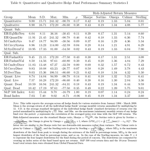
Generally, quantitative funds have a higher average return and a lower average standard deviation than qual funds. Amongst the quant funds, the highest average return comes from the Quantitative Directional strategy. The correlations of the fund categories with the S&P 500 are quite low at 0.17 and 0.38 for quant and qual respectively. The risk-adjusted return measures provide mixed evidence, but overall seems in favor of quant funds.

The qual funds perform significantly better than quant funds in up markets (25% and 15% respectively). However, the quant funds do significantly better in down markets (-2% versus -16%). This is mainly driven by the presence of Equity Market Neutral funds. In the 1990s, the average qual fund return was higher than the average quant fund return. They were roughly the same from 2000 – 2009. During the financial crisis (which we measure from January 2007 – March 2009), quant funds did better than qual funds (3.29% versus -4.77%).

Table 9 below shows performance summary statistics for the various funds:

Advantages and disadvantages of quantitative vs qualitative

Chincarini identifies several advantages quant funds hold over qualitative funds:

…the breadth of selections, the elimination of behavioral errors (which might be particularly important during the financial crisis of 2008 – 2009), and the potential lower administration costs (after hedge fund fees).

And several disadvantages:

The disadvantages for quantitative hedge funds include the reduced use of qualitative types of data, the reliance on historical data, the ability to quickly react to new economic paradigms. These three might have been especially crippling during the financial crisis of 2007 and 2009.

Finally, there is the potential of data mining, which will lead to strategies that aren’t as effective once implemented. In this paper, we will only focus on the return differences rather than attempting to detail which of the advantages or disadvantages in central in the return differences.

Hat tip Abnormal Returns.

Read Full Post »

The rationale for a quantitative approach to investing was first described by James Montier in his 2006 research report Painting By Numbers: An Ode To Quant:

  1. Simple statistical models outperform the judgements of the best experts
  2. Simple statistical models outperform the judgements of the best experts, even when those experts are given access to the simple statistical model.

In my experience, the immediate response to this statement in the investing context is always two-fold:

  1. What am I paying you for if I can build the model portfolio myself?
  2. Isn’t this what Long-Term Capital Management did?

Or, as Montier has it:

We find it ‘easy’ to understand the idea of analysts searching for value, and fund managers rooting out hidden opportunities. However, selling a quant model will be much harder. The term ‘black box’ will be bandied around in a highly pejorative way. Consultants may question why they are employing you at all, if ‘all’ you do is turn up and run the model and then walk away again.

It is for reasons like these that quant investing is likely to remain a fringe activity, no matter how successful it may be.

The response to these questions is as follows:

  1. It takes some discipline and faith in the model not to meddle with it. You’re paying the manager to keep his grubbly little paws off the portfolio. This is no small feat for a human being filled with powerful limbic system drives, testosterone (significant in ~50% of cases), dopamine and dopamine receptors and various other indicators interesting to someone possessing the DSM-IV-TR, all of which potentially lead to overconfidence and then to interference. You’re paying for the absence of interference, or the suppression of instinct. More on this in a moment.
  2. I’m talking about a simple model with a known error rate (momentarily leaving aside the Talebian argument about the limits of knowledge). My understanding is that LTCM’s problems were a combination of an excessively complicated, but insufficiently robust (in the Talebian sense) model, and, in any case, an inability to faithfully follow that model, which is failure of the first point above.

Suppressing intuition

We humans are clearly possessed of a powerful drive to allow our instincts to override our models. Andrew McAfee at Harvard Business Review has a recent post, The Future of Decision Making: Less Intuition, More Evidence, which essentially recapitulates Montier’s findings in relation to expertise, but McAfee frames it in the context of human intuition. McAfee discusses many examples demonstrating that intuition is flawed, and then asks how we can improve on intuition. His response? Statistical models, with a nod to the limits of the models.

Do we have an alternative to relying on human intuition, especially in complicated situations where there are a lot of factors at play? Sure. We have a large toolkit of statistical techniques designed to find patterns in masses of data (even big masses of messy data), and to deliver best guesses about cause-and-effect relationships. No responsible statistician would say that these techniques are perfect or guaranteed to work, but they’re pretty good.

And I love this story, which neatly captures the point at issue:

The arsenal of statistical techniques can be applied to almost any setting, including wine evaluation. Princeton economist Orley Ashenfleter predicts Bordeaux wine quality (and hence eventual price) using a model he developed that takes into account winter and harvest rainfall and growing season temperature. Massively influential wine critic Robert Parker has called Ashenfleter an “absolute total sham” and his approach “so absurd as to be laughable.” But as Ian Ayres recounts in his great book Supercrunchers, Ashenfelter was right and Parker wrong about the ’86 vintage, and the way-out-on-a-limb predictions Ashenfelter made about the sublime quality of the ’89 and ’90 wines turned out to be spot on.

Overall, we get inferior decisions and outcomes in crucial situations when we rely on human judgment and intuition instead of on hard, cold, boring data and math. This may be an uncomfortable conclusion, especially for today’s intuitive experts, but so what? I can’t think of a good reason for putting their interests over the interests of patients, customers, shareholders, and others affected by their judgments.

How do we proceed? McAfee has some thoughts:

So do we just dispense with the human experts altogether, or take away all their discretion and tell them to do whatever the computer says? In a few situations, this is exactly what’s been done. For most of us, our credit scores are an excellent predictor of whether we’ll pay back a loan, and banks have long relied on them to make automated yes/no decisions about offering credit. (The sub-prime mortgage meltdown stemmed in part from the fact that lenders started ignoring or downplaying credit scores in their desire to keep the money flowing. This wasn’t intuition as much as rank greed, but it shows another important aspect of relying on algorithms: They’re not greedy, either).

In most cases, though, it’s not feasible or smart to take people out of the decision-making loop entirely. When this is the case, a wise move is to follow the trail being blazed by practitioners of evidence-based medicine , and to place human decision makers in the middle of a computer-mediated process that presents an initial answer or decision generated from the best available data and knowledge. In many cases, this answer will be computer generated and statistically based. It gives the expert involved the opportunity to override the default decision. It monitors how often overrides occur, and why. it feeds back data on override frequency to both the experts and their bosses. It monitors outcomes/results of the decision (if possible) so that both algorithms and intuition can be improved.

Over time, we’ll get more data, more powerful computers, and better predictive algorithms. We’ll also do better at helping group-level (as opposed to individual) decision making, since many organizations require consensus for important decisions. This means that the ‘market share’ of computer automated or mediated decisions should go up, and intuition’s market share should go down. We can feel sorry for the human experts whose roles will be diminished as this happens. I’m more inclined, however, to feel sorry for the people on the receiving end of today’s intuitive decisions and judgments.

The quantitative value investor

To apply this quantitative approach to value investing, we would need to find simple quantitative value-based models that have outperformed the market. That is not a difficult process. We need go no further than the methodologies outlined in Oppenheimer’s Ben Graham’s Net Current Asset Values: A Performance Update or Lakonishok, Shleifer, and Vishny’s Contrarian Investment, Extrapolation and Risk. I believe that a quantitative application of either of those methodologies can lead to exceptional long-term investment returns in a fund. The challenge is making the sample mean (the portfolio return) match the population mean (the screen). As we will see, the real world application of the quantitative approach is not as straight-forward as we might initially expect because the act of buying (selling) interferes with the model.

Read Full Post »

« Newer Posts