Feeds:
Posts
Comments

Archive for the ‘Value Investment’ Category

I’m setting up a new experiment for 2009/2010 along the same lines as the 2008/2009 Net Net vs Activist Legend thought experiment pitting a little Graham net net against activist investing legend Carl Icahn (Net Net vs Activist Legend: And the winner is…). This time around I’m pitting a small portfolio of near Graham net nets against a small portfolio of ultra-low price-to-book value stocks. The reason? Near Graham net nets are stocks trading at a small premium to Graham’s two-thirds NCAV cut-off, but still trading at a discount to NCAV. While they are also obviously trading at a discount to book, they will in many cases trade at a higher price-to-book value ratio than a portfolio of stocks selected on the basis of price-to-book only. I’m interested to see which will perform better in 2010. The two portfolios are set out below (each contains 30 stocks). I’ll track the equal-weighted returns of each through the year.

The Near Graham Net Net Portfolio (extracted from the Graham Investor screen):

The Ultra-low Price-to-book Portfolio:

The Ultra-low Price-to-book Portfolio contains a sickly lot from a net current asset value perspective. Most have a negative net current asset value, as their liabilities exceed their current assets. Where that occurs, the proportion of price to NCAV is meaningless, so I’ve just recorded it as “N/A”. The few stocks that do have a positive net current asset value are generally trading a substantial premium to that value, with the exception of NWD and ZING, which qualify as Graham net nets.

While the Net Net vs Activist Legend thought experiment didn’t amount to (ahem) a formal academic study, there are two studies relevant to the outcome in that experiment: Professor Henry Oppenheimer’s Ben Graham’s Net Current Asset Values: A Performance Update, which found “[the] mean return from net current asset stocks for the 13-year period [from 1970 to 1983] was 29.4% per year versus 11.5% per year for the NYSE-AMEX Index.” Also relevant was Hedge Fund Activism, Corporate Governance, and Firm Performance, by Brav, Jiang, Thomas and Partnoy, in which the authors found that the “market reacts favorably to hedge fund activism, as the abnormal return upon announcement of potential activism is in the range of [7%] seven percent, with no return reversal during the subsequent year.”

This experiment is similar to the Net Net vs Activist Legend thought experiment in that it isn’t statistically significant. There are, however, several studies relevant to divining the outcome. In this instance, Professor Oppenheimer’s study speaks to the return on the Near Graham Net Net Portfolio, as Roger Ibbotson’s Decile Portfolios of the New York Stock Exchange, 1967 – 1984 (1986), Werner F.M. DeBondt and Richard H. Thaler’s Further Evidence on Investor Overreaction and Stock Market Seasonality (1987), Josef Lakonishok, Andrei Shleifer, and Robert Vishny’s Contrarian Investment, Extrapolation and Risk (1994) as updated by The Brandes Institute’s Value vs Glamour: A Global Phenomenon (2008) speak to the return on the Ultra-low Price-to-book Portfolio. One wrinkle in that theory is that the low price-to-book value studies only examine the cheapest quintile and decile, where I have taken the cheapest 30 stocks on the Google Finance screener, which is the cheapest decile of the cheapest decile. I expect these stocks to do better than the low price-to-book studies would suggest. That said, I expect that the Near Graham Net Net Portfolio will outperform the Ultra-low Price-to-book Portfolio by a small margin. Let me know which horse you’re getting on and the reason in the comments.

[Full Disclosure:  I hold RCMT and TSRI. This is neither a recommendation to buy or sell any securities. All information provided believed to be reliable and presented for information purposes only. Do your own research before investing in any security.]

Read Full Post »

In yesterday’s post we discussed some informal analysis I’ve undertaken on the returns to the quantitative investment strategy known as “High Minus Low” or HML. The first step was an analysis of HML’s components, high and low BM stocks. I described the HML strategy in some detail and analysed the long-term diminution in the returns to those components. I think that the returns to both high BM and low BM stocks have been attenuating significantly over time. The phenomenon persisted over whichever recent period I analysed (since 1926 to the present day, or over the last 25, 20, 15 or 10 years). This suggested that it’s got harder over time to earn excess returns as a value investor employing a high BM strategy.

In today’s post, I analyse the returns to HML at the strategy level and ask whether the returns to HML are really just returns to a levered high BM strategy. In a Goldman Sachs Asset Management (GSAM) presentation, Maybe it really is different this time, GSAM argued that the returns to HML have diminished since August 2007 because too many investors are employing the same  strategy, a phenomenon GSAM describe as “overcrowding.” In summary, I agree with GSAM’s view that the returns to HML have indeed stagnated since late 2007. I’m not sure that this is attributable to “overcrowding” as GSAM suggests or just a function of the underlying market performance of the components of HML (i.e. everything has been and continues to be expensive, leaving little room for good returns). Interestingly, even accounting for the period of low attenuated performance between August 2007 and the present, the HML strategy has performed reasonably well over the last 10 years, which has been a period of diminished (or non-existent) returns for equities. The returns to a 130/30 HML strategy over the last 10 years significantly outpaced a high BM strategy and the market in general. Surprisingly (to me at least), the low BM short didn’t add much to HML returns. This is especially surprising give that the period analysed was one where the low BM stocks bore the brunt of the collapse. That observation requires some further analysis, but it’s a prima facie argument that most of the returns to HML are due to the leverage inherent in the strategy.

Returns to HML

Most hedge fund strategies being proprietary and, hence, closely guarded secrets, I’m not sure what the typical HML strategy looks like. For the sake of this argument, I’ve constructed three HML portfolios. The first is 30% short the low BM decile and 130% long the high BM decile, which is a not uncommon hedge fund strategy. The second is 100% short the low BM decile and 100% long the high BM decile, which highlights the low BM short and removes the effects of leverage from the high BM long. The third is 130% long the High BM decile and has no short, to remove the effect of the short and highlight the effect of the leverage. How would those strategies have fared over the last 10 years, which, as we saw yesterday, was a period of attenuated returns for equities?

The 130/30 HML strategy

“Low BM” is the lowest BM decile, marked in red. This is Decile 1 from the Average monthly returns to decile BM portfolios chart in yesterday’s post. “High BM” is the highest BM decile, marked in blue. This is Decile 1o from yesterday’s chart. The green “HML” line is -30% of the return on the low BM decile and 130% the return on the high BM decile. “Delta,” in purple, is the difference between the return on the low and high BM components of the HML strategy. Here’s the chart:

Several observations can be made about the chart. First, as at September 2009, the “Low BM” strategy (in red) is down 3%, which approximates the return on the market as a whole over the last 10 years. The “High BM” strategy (in blue) is up about 95%, which is not a great return over 10 years, but well ahead of the market in general and the Low BM portfolio. The HML portfolio is up around 124%, well ahead of both the Low BM and High BM portfolios. As recently as 2003, the 130/30 HML portfolio was underwater and it nearly accomplished this feat again in 2009. It performed almost in line with the High BM portfolio while the market was tanking, which is when I would have expected the Low BM short to protect the return on the HML, affording only a little protection. It seems that the return on the 130% long component of the High BM portfolio caused the HML strategy to tank with the High BM portfolio, although it also caused it to recover much faster. While GSAM is correct that HML returns have been reduced since late 2007, the 10-year return on the 130/30 HML is attractive.

The 100/100 HML strategy

In this chart the green “HML” line is -100% of the return on the low BM decile and 100% the return on the high BM decile:

The 100/100 HML chart illustrates several points. First, as at September 2009, the HML portfolio is up 98%, in line with the High BM portfolio. Where the Low BM portfolio falls, the 100% low BM short in the HML protects it. For the last 10 years, it has generally protected the HML return. Of course it hurts the HML’s performance when the low BM short rises, which, as we saw yesterday, has generally been the case since 1926.

The Levered High BM strategy

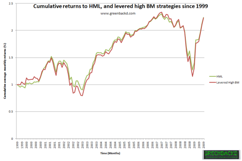
This chart shows the High BM portfolio levered at the same rate as the 130/30 HML strategy (i.e.130%), but without the low BM short:

The Levered High BM portfolio tracks (visually) almost identically to the 130/30 HML strategy (Levered High BM closed up 123%, HML closed up 124%). This suggests to me that most of the additional gains in the 130/30 HML strategy over the High BM strategy are simply attributable to the leverage in the HML, and not out of any protection afforded by the low BM short.

Recent returns to HML depressed

A casual perusal of any chart above illustrates that HML has not progressed since August 2007. GSAM argues that this is a secular phenomenon due to overcrowding. I’m not convinced that it’s a secular phenomenon, but it’s certainly noteworthy. I’m also not entirely convinced that it’s due to overcrowding. It could just as easily be a function of the high price for equities in August 2007 and again now. GSAM argues that your view on the phenomenon as being either cyclical or secular is key to how you position yourself for the future. If you believe it’s cyclical, you’re a “Sticker,” and, if you believe it’s secular, you’re an “Adapter”. The distinction, according to Zero Hedge, is as follows:

The Stickers believe this is part of the normal volatility of such strategies

• Long-term perspective: results for HML (High Book-to-Price Minus Low Book-to-Price) and WML (Winners Minus Losers) not outside historical experience

• Investors who stick to their process will end up amply rewarded

The Adapters believe that quant crowding has fundamentally changed the nature of these factors

• Likely to be more volatile and offer lower returns going forward

• Need to adapt your process if you want to add value consistently in the future

I’m in the cyclical camp, but it may be other players withdrawing from the field that causes the cycle to turn.

Conclusion

Despite GSAM’s protestations to the contrary, and despite the diminution of equity returns at both the value and glamour ends of the market, HML remains an attractive strategy. Over a 10-year period of attenuated equity returns, a 130/30 HML strategy performed very well. It seems, however, that most of the returns to the 130/30 strategy are attributable to the leverage in the high BM portfolio, rather than any protection in the low BM short. As we saw yesterday, the low BM decile, while generating a lower return than the high BM decile over time, has mainly generated positive returns. This means that the low BM short will generally hurt the HML strategy’s performance.

My vast preference remains a leverage-free, long-only, ultra-high BM portfolio for a variety of reasons not connected with the chronic underperformance of the short, most notably that it’s the lowest risk portfolio available (despite what Fama and French say). In my opinion, the diminution in returns to the high BM strategy we observed yesterday is a cyclical phenomenon. 25 years is a long time for a cycle to turn, but I’m reasonably confident that the high BM strategy will again generate average monthly returns in line with the long-run average on yesterday’s chart, which means average monthly returns in the vicinity of 1.2% to 1.4%. I don’t foresee this occurring any time soon, and I think dwindling returns are the order of the day for the next 5 or 10 years. If I had to be anywhere in equities, however, I’d start in the cheapest decile of the market on a price-to-book basis and work my way through to those with the highest proportion of current assets. That’s a proven strategy that served Graham and Schloss very well, and, as far as I can see, there’s no reason why it shouldn’t continue to work.

Read Full Post »

Recently we discussed a Goldman Sachs Asset Management (GSAM) presentation, Maybe it really is different this time, in which GSAM argued that High Minus Low or HML, a quantitative investment strategy that seeks to profit from the performance differential between high and low book value-to-market value (BM) stocks, had underperformed since August 2007 due to “overcrowding.” Robert Litterman, Goldman Sachs’ Head of Quantitative Resources, was quoted as saying that “strategies such as those which focus on price rises in cheaply-valued stocks…[have] become very crowded” since August 2007 and therefore unprofitable. The GSAM presentation included a variety of slides showing the reduction in the returns to HML and the growth in the number of practitioners in the space (See my summary of the GSAM presentation and Zero Hedge’s take on it).

Over the last week I’ve run my own informal analysis of the returns to HML and its components, high and low BM stocks. The resulting post has metastasised into an epic (by my standards), so I’ve broken it into two parts, Component returns (Part 1) and HML returns (Part 2). In today’s post, Component returns, I describe the HML strategy in some detail and analyse the long-term diminution in the returns to the components of HML, namely, high BM (low P/B) stocks and low BM (high P/B) stocks. The results are stunning. The returns to the high BM and low BM stocks have been attenuating significantly over time. Further, the phenomenon persists over whichever recent period we elect to choose (since 1926, or the last 25 years, 20 years, 15 years or 10 years). This suggests that it’s got harder over time to earn excess returns as a value investor employing a high BM strategy.

In tomorrow’s post, I analyse the returns to HML at the strategy level and ask whether the returns to HML are really just returns to a levered high BM strategy. In summary, the returns to HML have indeed stagnated since late 2007. I’m not sure that this is attributable to “overcrowding” as GSAM suggests or just a function of the underlying market performance of the components of HML (i.e. everything has been and continues to be expensive, leaving little room for good returns). Interestingly, GSAM’s argument that HML is dead as of August 2007 aside, the HML strategy has performed reasonably well over the last 10 years, which has been a period of diminished (or non-existent) returns for equities. The returns to a 130/30 HML strategy over the last 10 years significantly outpace a high BM strategy and the market in general. Surprisingly (to me at least), the low BM short didn’t add much to HML returns. This is especially surprising give that the period analysed was one where the low BM stocks bore the brunt of the collapse. That observation requires some further analysis, but it’s a prima facie argument that most of the returns to HML are due to the leverage inherent in the strategy.

A primer on HML

As I mentioned above, HML is a quantitative investment strategy that seeks to profit from the performance differential between high and low book value-to-market value stocks. It’s interesting to me because it appears to be a value-based strategy. In actuality, it finds its roots in the Fama and French Three-Factor Model, which is an attempt to explain the excess returns attributable to value stocks within an efficient markets context. HML also owes an intellectual debt to the various studies demonstrating the relative outperformance of low price-to-value stocks over higher price-to-value stocks – Roger Ibbotson’s Decile Portfolios of the New York Stock Exchange, 1967 – 1984 (1986), Werner F.M. DeBondt and Richard H. Thaler’s Further Evidence on Investor Overreaction and Stock Market Seasonality (1987), Josef Lakonishok, Andrei Shleifer, and Robert Vishny’s Contrarian Investment, Extrapolation and Risk (1994) as updated by The Brandes Institute’s Value vs Glamour: A Global Phenomenon (2008) – but it is most closely associated with Fama and French.

Fama and French observed in their 1992 paper, The Cross-Section of Expected Stock Returns, that there is “striking evidence” of a “strong positive relation between average return and book-to-market equity” [“BE” is book equity and “ME” is market equity, so “BE/ME” is just BM, the inverse of P/B]:

Average returns rise from 0.30% for the lowest BE/ME portfolio to 1.83% for the highest, a difference of 1.53% per month.

Note also that the strong relation between book-to-market equity and average return is unlikely to be a [beta] effect in disguise.*

[Although] BE/ME has long been touted as a measure of the return prospects of stocks, there is no evidence that its explanatory power deteriorates through time. The 1963-1990 relation between BE/ME and average return is strong, and remarkably similar for the 1963-1976 and 1977-1990 subperiods. Second, our preliminary work on economic fundamentals suggests that high-BE/ME firms tend to be persistently poor earners relative to low-BE/ME firms.

Ibbotson (1986), DeBondt and Thaler (1987), Lakonishok, Shleifer, and Vishny (1994) and The Brandes Institute (2008) all make similar findings. Low P/B stocks outperform higher P/B stocks in the aggregate, and in rank order, the cheapest decile, quintile, quartile etc outperforming the next cheapest and so on. This phenomenon obviously presents a problem for the efficient markets crowd because the historic excess returns of value stocks over glamour stocks cannot be explained by the traditional CAPM model. Fama and French’s solution is the Three-Factor Model.

Fama and French attribute the variation in average returns between high and low BM stocks to “relative distress,” arguing that value strategies (i.e. high BM stocks) produce abnormal returns because they are fundamentally riskier. This observation is the impetus for the inclusion of “value” as a factor in Fama and French’s Three-Factor Model, where it is accounted for as “HML”. (It was also the impetus for Piotroski’s F_SCORE, which seeks to use “context-specific financial performance measures to differentiate strong and weak firms” within the universe of high BM stocks.)

HML in the Fama and French context measures the historic excess returns of value stocks over growth stocks, which break the traditional CAPM model. Here’s how they circumvent the problem: By splitting out HML from the market return and labelling the portion of the excess return attributable to HML as “riskier,” Fama and French can explain away those excess returns. They then simply apply an HML coefficient to a portfolio of value stocks and – abracadabra – the expected return is higher than the market return but explainable within the efficient markets world because of the additional risk attributable to value. The proponents of the efficient markets hypothesis breathe a sigh of relief and continue to believe that no one can make excess returns once those returns are adjusted for risk. (Don’t mention that value is not, per se, riskier, because such an observation would break the model all over again.) It’s worth noting that Lakonishok, Shleifer, and Vishny (1994) disagree with Fama and French’s assertion that the returns are due to financial distress, arguing instead that the returns to value are the result of a bias that leads investors to extrapolate past performance too far into the future, not fully appreciating the phenomenon of mean reversion.

Whatever the basis for the returns to value, the phenomenon has attracted a substantial following in the world of quantitative investing. So much so that GSAM thinks the field is now “overcrowded” and that explains the diminution in returns since August 2007. The attraction of the HML strategy to a quant is easy to understand: They’re agnostic to the reason for the excess returns, and more than happy to earn some and remain market neutral. The solution is to split out from the market return the excess return attributable to HML. How does one do that in practice? One simply buys the value stocks and sells the glamour stocks. This means buying high BM stocks and selling short low BM stocks. It’s extraordinary that, despite the tortured EMH reasoning, HML is a strategy that a value investor would recognize and (shorting, leverage and aggregation notwithstanding) probably approve of in its general terms. Before looking at the returns to the HML strategy, I think it’s useful to look under the hood and consider the “engine” of the strategy, which is the returns to the underlying components.

* One of the observations made by Fama and French (1992) is that “average returns for negative BE firms are high, like the average returns of high BE/ME firms. Negative BE (which results from persistently negative earnings) and high BE/ME (which typically means that stock prices have fallen) are both signals of poor earnings prospects.” This is very interesting. I’ve never heard of a negative BM strategy. While it makes me a little nervous to think about, it’s possible that negative BM stocks are an untapped source of returns. Perhaps it’s just the leverage at the company level, but it warrants a further investigation and a later post. Let me know if you’ve got any data or studies on the subject.

Returns to HML’s components: High BM and Low BM

There are two components to the HML strategy: The high BM long and the low BM short. The strategy seeks to remain market neutral by selling short low BM stocks, which are expected to fall back to the mean market BM value, and using leverage to buy high BM stocks, which are expected to rise to the mean market BM value. To see how each component performs, I’ve produced a chart of average monthly stock returns since 1926. Before I present the graph, a quick disclaimer: What follows does not amount to a formal academic study into the relative performance of high BM and low BM over time. It’s nothing more than me messing around with COMPUSTAT return data and plugging it into an Excel spreadsheet. Stocks were divided into ten deciles based on book value-to-market value. Average returns for each decile were calculated on a monthly basis over five different time periods:

  • “All” from July 1926 to September 2009
  • “25 Years”, from October 1984 to September 2009
  • “20 Years”, from October 1989 to September 2009
  • “15 Years”, from October 1994 to September 2009
  • “10 Years”, from October 1999 to September 2009

“Decile 10” is formed from the portfolio of stocks with the highest BM ratio (lowest P/B), “Decile 1” is the portfolio of stocks with the lowest BM ratio (highest P/B) and so on. Here’s the chart:

For me, three observations leap out from the chart. First, the relationship between high and low BM deciles is relatively unchanged over time. The relatively high BM stocks in deciles 10, 9, and 8 tend to outperform the relatively lower BM stocks in deciles 1, 2, and 3. With few exceptions, the higher the ratio of book to market, the better the performance.

Second, the returns to all deciles have attenuated significantly over time. This was one of the questions I had after reading The Brandes Institute’s Value vs Glamour: A Global Phenomenon update of the Contrarian Investment, Extrapolation and Risk. The Brandes Institute paper didn’t split out from Lakonishok, Shleifer, and Vishny’s paper the more recent returns to high BM stocks, but the blended return was lower in the later study, suggesting that returns had diminished in the intervening period. As far as this simple analysis goes, it seems to confirm that impression.

The third observation is that the low BM decile – Decile 1 – has for most of the time had a positive monthly return. It is only over the last 10 years that the monthly returns for the lowest BM decile have been negative. This is significant because this means that, the last 10 years aside, one employing the HML strategy would have lost money on the low BM short, and would have earned better returns without the short. Over the last 10 years, however, one would expect that the low BM short has paid off handsomely. As you’ll see tomorrow, this is not actually the case.

Hat tip to the Ox for the return data.

Read Full Post »

The wonderful Miguel Barbosa of Simoleon Sense has interviewed Joe Calandro, Jr., author of Applied Value Investing. The interview is first class. Joe Calandro, Jr. is an interesting guy. Deep value? Check. Activist investing? He’s for it. Austrian School of Economics? Check. I think I just wet myself.

Here’s Joe’s take on value:

Q. Can you give me an example of some of your best investments?

A. In the book I profile a value pattern that I call “base case value” which is simply net asset value reconciling with the earnings power value. Firms exhibiting that pattern, which sell at reasonable margins of safety have proved highly profitable to me. In the book, I show examples of this type of investment.

“Value investing” in general has 3 core principles:

(1) The circle of competence, which essentially relates to an information advantage and holds that you will do better if you stick to what you know more about than others.

(2) The principle of conservatism. You will have greater faith in valuations if you prepare them conservatively.

(3) The margin of safety. You should only invest if there is a price-to-value gap: when the gap disappears you exit the position.

Here’s Joe on activist investing:

Q. You’re primarily in the corporate sector now; in your book you touch upon the failure of corporate M&A groups to apply value investing.  Why do you think this is the case? What is your take on activist value investors?

A. That’s a good question and I don’t have a definitive answer for it. My take on it is that Corporate America hasn’t been trained in Graham and Dodd. For example, if you get away from Columbia and some of the other top schools you really don’t have courses of study based on Graham and Dodd. I think this lack of education carries over to practice. If educational institutions aren’t teaching something, then executives are going to have a difficult time applying it. And if they do try to apply it, their employees and boards may not understand it. Hopefully, my book will help to rectify this over time.

Regarding activist investors, I think every investor should be active. If you allocate money to a security (either equity or debt) you have the responsibility of becoming involved in the respective firm because, as Benjamin Graham noted, you invested in a business, not in a piece of paper or a financial device. This is real money in real businesses so there is a responsibility that comes with investing.

And Joe’s view on economics:

Q. Can you give us a tour of the major insights you obtained from the Austrian School of Economics.

A. I have two big academic regrets: I did not study Graham and Dodd or Austrian economics until I was in my mid 30’s. One of the major theories of Austrian economics is its business cycle theory. Just the other day (11/6/2009), that theory was mentioned in the WSJ by Mark Spitznagel, who is Nassim Taleb’s partner, in his article “The Man Who Predicted the Depression.” As you know, Taleb has also spoken highly of Austrian economics as have other successful traders/practitioners such as Victor Sperandeo, Peter Schiff and Bill Bonner.

Austrian economics finds success with practitioners because, I think, Austrian economists are truly economists; they do not try to be applied mathematicians. Therefore, Austrians tend to see economics for what it is; namely, a discipline built around general principles that can be applied broadly to economic phenomena. As a result, Austrian economics is generally very useful in areas such as the business cycle and the consequences of government intervention, which are very pertinent topics today.

Read the rest of the interview while I run out to buy the book.

Read Full Post »

Greenbackd is a proud sponsor of the 2010 5th Annual Value Investing Congress West and I’ve been able to secure a special discount for you to attend.

Though the Congress is more than 6 months away, over 40% of the seats have already been reserved. Register by midnight next Tuesday, December 15, 2009 with discount code P10GB1 and you’ll save $1,750 off the regular price of admission.

Every year hundreds of people from around the world converge at this not-to-be-missed event to network with other savvy, sophisticated investors and learn from some of world’s most successful money managers. At the upcoming event, all-star investors will share their thoughts on today’s tumultuous markets and present their best, actionable investment ideas. Just one idea could earn you outstanding returns.

Here are Jon Heller’s notes on Lloyd Khaner of Khaner Capital’s talk at this year’s event:

The Key to Turnarounds

First time presenter at the Value Investing Congress, Khaner, who has compounded 445.4% since 1991 (versus 295.2% for the S&P 500), looks for the following attributes in potential investments:

  • Unique management
  • Strong decision making ability
  • Avoid value traps
  • Debt/Equity less than 70%
  • Avoid dying industries
  • Franchise companies with manageable debt

Khaner is a big believer in the concept of “CEO family trees,”placing value on those that have been trained or worked under other successful CEO’s.

Khaner listed the signs of a successful turnaround, including:

  • Cutting unprofitable sales
  • Cutting headcount
  • New senior managers
  • Fix customer relationships
  • CEO sets plan within 3 months
  • Gross Margin up
  • SG&A down
  • Focus on Return on Capital
  • Restructure Debt-Push out maturities.

One of Khaner’s favorite ideas is Starbucks (SBUX):

  • Slowing new store openings
  • Improving service
  • Expects positive comps fiscal 2010
  • ROIC growth 100-200 bps next 3+ years
  • FCF $500-$750 million 3+ years

See a slide show of the last Value Investing Congress in New York.

Don’t miss your opportunity to learn from these financial luminaries. The insights you gain could guide your investment decisions for years to come. Remember, you must register by midnight December 15, 2009 with discount code P10GB1 to take advantage of this special offer and SAVE $1,750 off the regular price to attend. Avoid disappointment – reserve your seat today.

Read Full Post »

It seems to me counterintuitive that book value should be useful as a value metric. Book value, after all, is a historical accounting measure of a company’s balance sheet. It has nothing to do with “intrinsic value,” which is the measure conceived by John Burr Williams in his 1938 treatise The Theory of Investment Value. Warren Buffett is a well-known proponent of “intrinsic value.” In his 1992 letter to shareholders he provided the following explication of the concept:

In The Theory of Investment Value, written over 50 years ago, John Burr Williams set forth the equation for value, which we condense here: The value of any stock, bond or business today is determined by the cash inflows and outflows – discounted at an appropriate interest rate – that can be expected to occur during the remaining life of the asset. Note that the formula is the same for stocks as for bonds. Even so, there is an important, and difficult to deal with, difference between the two: A bond has a coupon and maturity date that define future cash flows; but in the case of equities, the investment analyst must himself estimate the future “coupons.” Furthermore, the quality of management affects the bond coupon only rarely – chiefly when management is so inept or dishonest that payment of interest is suspended. In contrast, the ability of management can dramatically affect the equity “coupons.”

The investment shown by the discounted-flows-of-cash calculation to be the cheapest is the one that the investor should purchase – irrespective of whether the business grows or doesn’t, displays volatility or smoothness in its earnings, or carries a high price or low in relation to its current earnings and book value. Moreover, though the value equation has usually shown equities to be cheaper than bonds, that result is not inevitable: When bonds are calculated to be the more attractive investment, they should be bought.

Buffett’s explanation draws a sharp distinction between intrinsic value and book value – “The investment shown by the discounted-flows-of-cash calculation to be the cheapest is the one that the investor should purchase – irrespective of whether the business…carries a high price or low in relation to its…book value.” While Buffett’s statement may be true, that does not mean that book value is useless as a value metric. Far from it. As the various studies we have discussed recently demonstrate – Roger Ibbotson’s Decile Portfolios of the New York Stock Exchange, 1967 – 1984 (1986), Werner F.M. DeBondt and Richard H. Thaler’s Further Evidence on Investor Overreaction and Stock Market Seasonality (1987), Josef Lakonishok, Andrei Shleifer, and Robert Vishny Contrarian Investment, Extrapolation and Risk (1994) and The Brandes Institute’s Value vs Glamour: A Global Phenomenon (2008) – low price-to-book value stocks outperform higher priced stocks and the market in general. Why might that be so?

In Contrarian Investment, Extrapolation and Risk, Lakonishok, Shleifer, and Vishny frame their findings in the context of contrarianism, what I like to call the Ricky Roma style of investing:

I subscribe to the law of contrary public opinion. If everyone thinks one thing, then I say, “Bet the other way.”

The problem, as I see it, with low price-to-book investment is that the strategy always flashes a buy signal. When the market is getting very toppy, you can still find the cheapest decile, quintile, quartile, or whatever on a price-to-book basis to buy. That decile might not recede as much as the market in general, but I’d bet odds on that it will still recede. That might not be a problem if, in the aggregate, the price-to-book strategy is able to generate satisfactory long-term returns. A better strategy, however, would remove the opportunities to trade as the market gets expensive, forcing you to sit in cash. I believe this is why Piotroski’s F_SCORE and Graham’s Net Current Asset Value strategies perform so well. When the market gets expensive, those opportunities disappear.

The American Association of Individual Investors website offers various value and growth screens to its membership. Piotroski’s F_SCORE is one such screen. The AAII reports that, of the 56 screens it offers, the only screen that had positive results in 2008 was Piotroski’s F_SCORE (via Forbes):

Believe it or not, the five stocks that AAII bought using Piotroski’s strategy in 2008 gained 32.6% on average through the end of the year. The median performance for all of the AAII strategies last year? -41.7%.

It’s clearly an austere screening criteria if it only lets a handful of stocks get through when the market is high, and in this respect very similar to Graham’s Net Current Asset Value strategy. Right now it has one stock on its screen. That stock? Tune in next week for the full analysis. (I’m starting to sound like The Motley Fool).

Read Full Post »

Carl Icahn recently gave a guest lecture to Professor Robert Shiller’s Yale Financial Markets class.

In the lecture, Icahn talks about how he started out in finance and evolved into a shareholder activist. He trots out a few of his old saws: the biggest challenge facing corporate America is weak management and today’s CEOs, with exceptions, might not be the most capable of leading global companies. He also discusses the economy and slaps down an undergrad Yalie who has the temerity to have him repeat an answer, which is fun to watch. There are a few gems, including this one:

I was borrowing money and bought all these convertibles and I thought I was a genius and Jack Dreyfus said, you’re going to lose all your money. I had made a few bucks playing poker and that’s how I started with about eight, ten thousand dollars and I made all this money by borrowing at 90%. I would go out and I was making a lot more in two weeks than my father made in two years. My father said, well you know, put the money away. I said, no Dad, I’m really going to make a fortune here. So, I went out–I remember once–and bought a Galaxy convertible. It was a beautiful car. I had a beautiful girlfriend; she was a model–it was just pretty nice.

What happened? The crash came in 1962. I was wiped out in one day; I didn’t even have the poker winnings left. I tell you, I can’t recall if the car left first or the girl left first, but it was pretty close–maybe the same day actually. After that, I learned you have to learn something and I became an expert in options.

Here’s Icahn on his investment strategy:

What I do today still is pretty much the same idea. You buy stocks in a company that is cheap and you look at the asset value of the companies that you buy the stocks in and it becomes a little more complex. Basically, you look for the reason that they’re really cheap and the major reason is often–and usually–very poor management. In a sense, it’s like an arbitrage. You go in; you buy a lot of stock in a company; and you then try to make changes at the company. Today, if you read the newspapers tomorrow, you’ll read–we’re trying to do the same thing at Motorola and if you bother to read The Wall Street Journal tomorrow–or maybe The Times, I don’t know–you’ll see a little bit of what we’re trying to do there. We’re trying to get them to change the structure of the company. We think the board is a very poor board there and we’re trying to change what happens.

And, finally, Icahn responding to a question about activism:

Student: Hi, Mr. Icahn. One major criticism that one CEO against corporate activist that they think activists don’t think long-term interest of the corporation; they just want to get money and get out. How do you answer to that?

Icahn: I would just say that the facts don’t bear that out as far as I’m concerned. I mean, if you–I own quite a few companies. Any company we got control of I put literally hundreds of millions of dollars into them. I mean, I bought a company in 1985–a rail car company–we put hundreds of millions; we still have the fleet. I bought casinos and energy companies and over the years kept them; sold them now, but that’s after ten years. So, any company that we’ve been able to get control of I actually kept. Because getting control is a great thing. If you really believe that management’s not doing well, you can go and clean them up and put a good guy in, So, we–I know they criticize you like that, but that’s part of the propaganda machine; but it’s just not the facts.

Student: A related question is that, what do you do when your activist spirit is not appreciated, as in the case of Motorola when you asked for a seat on the board but just get declined? What’s your next step?

Icahn: Alright, you have patience and now it’s a year later and we’ll see what happens now. Motorola is a good example of what I’m talking about. People don’t like it; they don’t like the cell phone business, but I really think that that business, if you look at Motorola and study it, you’re buying that whole business for nothing. It’s not reflected in the stock price, but they have to do it. As I said publicly, take that business out of Motorola; spin it off and give it to the shareholders. I think, then, you’ve got a real good value. What I’m saying is, nobody likes it now, but hopefully I’m correct on that. I really think by being an activist and putting pressure on that board that has done nothing, really–I think eventually that will happen, hopefully.

Hat tip Mark.

Read Full Post »

The phenomenal Zero Hedge has an article, Goldman Claims Momentum And Value Quant Strategies Now Overcrowded, Future Returns Negligible, discussing Goldman Sachs head of quantitative resources Robert Litterman’s view that  “strategies such as those which focus on price rises in cheaply-valued stocks…[have] become very crowded” since August 2007 and therefore unprofitable. The strategy to which Litterman refers is “HML” or “High Book-to-Price Minus Low Book-to-Price,” which is particularly interesting given our recent consideration of the merits of price-to-book value as an investment strategy and the various methods discussed in the academic literature for improving returns from a low P/B strategy. Litterman argues that only special situations and event-driven strategies that focus on mergers or restructuring provide opportunities for profit:

What we’re going to have to do to be successful is to be more dynamic and more opportunistic and focus especially on more proprietary forecasting signals … and exploit shorter-term opportunistic and event-driven types of phenomenon.

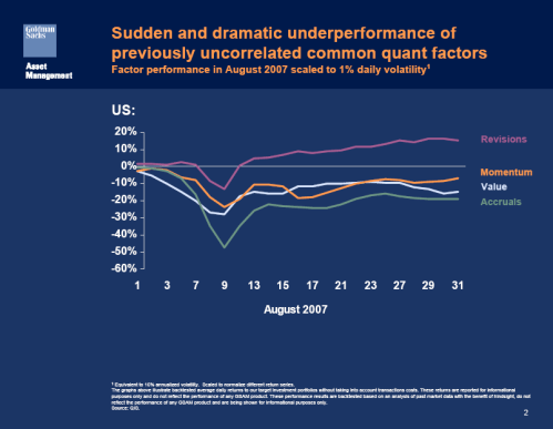
In a follow-up article, More On The Futility Of Groupthink Quant Strategies, And Why Momos Are Guaranteed To Lose Money Over Time, Zero Hedge provides a link to a Goldman Sachs Asset Management presentation, Maybe it really is different this time (.pdf via Zero Hedge), from the June 2009 Nomura Quantitative Investment Strategies Conference. The presentation supports Litterman’s view on the underperformance of HML since August 2007. Here’s the US:

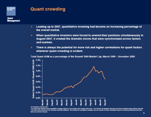
Here’s a slide showing the ‘overcrowding” to which Litterman refers:

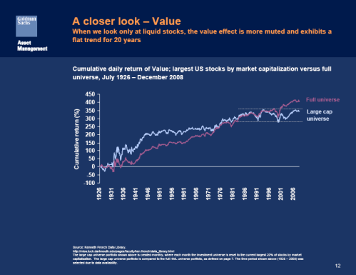
And its effect on the relative performance of large capitalization value to the full universe:

The returns get really ugly when transaction costs are factored into the equation:

A factor decay graph showing the decline in legacy portfolios relative to current portfolios, lower means and faster decay indicating crowding:

Goldman says that there are two possible responses to the underperformance, and characterizes each as either a “sticker” or an “adapter.” The distinction, according to Zero Hedge, is as follows:

The Stickers believe this is part of the normal volatility of such strategies

• Long-term perspective: results for HML (High Book-to-Price Minus Low Book-to-Price) and WML (Winners Minus Losers) not outside historical experience

• Investors who stick to their process will end up amply rewarded

The Adapters believe that quant crowding has fundamentally changed the nature of these factors

• Likely to be more volatile and offer lower returns going forward

• Need to adapt your process if you want to add value consistently in the future

In Contrarian Investment, Extrapolation, and Risk, Josef Lakonishok, Andrei Shleifer, and Robert Vishny argued that value strategies produce superior returns because most investors don’t fully appreciate the phenomenon of mean reversion, which leads them to extrapolate past performance too far into the future. Value strategies “exploit the suboptimal behavior of the typical investor” by behaving in a contrarian manner: selling stocks with high past growth as well as high expected future growth and buying stocks with low past growth and as well as low expected future growth. It makes sense that crowding would reduce the returns to a contrarian strategy. Lending further credence to Litterman and Goldman’s argument is the fact that the underperformance seems to be most pronounced in the large capitalization universe (see the “A closer look – value” slide) where the larger investors must fish. If you’re not forced by the size of your portfolio to invest in that universe it certainly makes sense to invest where contrarian returns are still available. Special situations like liquidations and event-driven investments like activist campaigns offer a place to hide if (and when) the market resumes the long bear.

My firm Acquirers Funds® helps you put the acquirer’s multiple into action. Click here to learn more about our deep value strategy.

Read Full Post »

The second method for boosting the performance of book value as a predictor of future investment returns is Joseph D. Piotroski’s elegant F_SCORE. Piotroski first discussed his F_SCORE in 2002 in Value Investing: The Use of Historical Financial Statement Information to Separate Winners from Losers. In the paper, Piotroski examines whether the application of a simple accounting-based fundamental analysis strategy to a broad portfolio of high book-to-market firms can improve the returns earned by an investor. Piotroski found that his method increased the mean return earned by a low price-to-book investor “by at least 7 1/2% annually” through the “selection of financially strong high BM firms.”

In addition, an investment strategy that buys expected winners and shorts expected losers generates a 23% annual return between 1976 and 1996, and the strategy appears to be robust across time and to controls for alternative investment strategies.

With a return of that magnitude, it’s well worth a deeper look.

Piotroski’s rationale

Piotroski uses “context-specific financial performance measures to differentiate strong and weak firms:”

Instead of examining the relationships between future returns and particular financial signals, I aggregate the information contained in an array of performance measures and form portfolios on the basis of a firm’s overall signal. By focusing on value firms, the benefits to financial statement analysis (1) are investigated in an environment where historical financial reports represent both the best and most relevant source of information about the firm’s financial condition and (2) are maximized through the selection of relevant financial measures given the underlying economic characteristics of these high BM firms.

F_SCORE

On the assumption that the “average high BM firm is financially distressed,” Piotroski chose nine fundamental signals to measure three areas of the firm’s financial condition: profitability, financial leverage/liquidity, and operating efficiency:

In this paper, I classify each firm’s signal realization as either “good” or “bad,” depending on the signal’s implication for future prices and profitability. An indicator variable for the signal is equal to one (zero) if the signal’s realization is good (bad). I define the aggregate signal measure, F_SCORE, as the sum of the nine binary signals. The aggregate signal is designed to measure the overall quality, or strength, of the firm’s financial position, and the decision to purchase is ultimately based on the strength of the aggregate signal.

F_SCORE component: Profitability

On the basis that “current profitability and cash flow realizations provide information about the firm’s ability to generate funds internally,” Piotroski uses four variables to measure these performance-related factors: ROA, CFO, [Delta]ROA, and ACCRUAL:

I define ROA and CFO as net income before extraordinary items and cash flow from operations, respectively, scaled by beginning of the year total assets. If the firm’s ROA (CFO) is positive, I define the indicator variable F_ROA (F_CFO) equal to one, zero otherwise. I define ROA as the current year’s ROA less the prior year’s ROA. If [Delta]ROA [is greater than] 0, the indicator variable F_[Delta]ROA equals one, zero otherwise.

I define the variable ACCRUAL as current year’s net income before extraordinary items less cash flow from operations, scaled by beginning of the year total assets. The indicator variable F_ ACCRUAL equals one if CFO [is greater than] ROA, zero otherwise.

F_SCORE component: Leverage, liquidity, and source of funds

For the reason that “most high BM firms are financially constrained” Piotroski assumes that an increase in leverage, a deterioration of liquidity, or the use of external financing is a bad signal about financial risk. Three of the nine financial signals are therefore designed to measure changes in capital structure and the firm’s ability to meet future debt service obligations: [Delta]LEVER, [Delta]LIQUID, and EQ_OFFER:

[Delta]LEVER seeks to capture changes in the firm’s long-term debt levels:

I measure [Delta]LEVER as the historical change in the ratio of total long-term debt to average total assets, and view an increase (decrease) in financial leverage as a negative (positive) signal. By raising external capital, a financially distressed firm is signaling its inability to generate sufficient internal funds (e.g., Myers and Majluf 1984, Miller and Rock 1985). In addition, an increase in long-term debt is likely to place additional constraints on the firm’s financial flexibility. I define the indicator variable F_LEVER to equal one (zero) if the firm’s leverage ratio fell (rose) in the year preceding portfolio formation.

[Delta]LIQUID seeks to measure the historical change in the firm’s current ratio between the current and prior year, where Piotroski defines the current ratio as the ratio of current assets to current liabilities at fiscal year-end:

I assume that an improvement in liquidity (i.e., [Delta]LIQUID [is greater than] 0) is a good signal about the firm’s ability to service current debt obligations. The indicator variable F_[Delta]LIQUID equals one if the firm’s liquidity improved, zero otherwise.

Piotroski argues that financially distressed firms raising external capital “could be signaling their inability to generate sufficient internal funds to service future obligations” and  the fact that these firms are willing to issue equity when their stock prices are depressed “highlights the poor financial condition facing these firms.” EQ_OFFER captures whether a firm has issued equity in the year preceding portfolio formation. It is set to one if the firm did not issue common equity in the year preceding portfolio formation, zero otherwise.

F_SCORE component: Operating efficiency

Piotroski’s two remaining signals seek to measure “changes in the efficiency of the firm’s operations:” [Delta]MARGIN and [Delta]TURN. Piotroski believes these ratios are important because they “reflect two key constructs underlying a decomposition of return on assets.”

Piotroski defines [Delta]MARGIN as the firm’s current gross margin ratio (gross margin scaled by total sales) less the prior year’s gross margin ratio:

An improvement in margins signifies a potential improvement in factor costs, a reduction in inventory costs, or a rise in the price of the firm’s product. The indicator variable F_[Delta]MARGIN equals one if [Delta]MARGIN is positive, zero otherwise.

Piotroski defines [Delta]TURN as the firm’s current year asset turnover ratio (total sales scaled by beginning of the year total assets) less the prior year’s asset turnover ratio:

An improvement in asset turnover signifies greater productivity from the asset base. Such an improvement can arise from more efficient operations (fewer assets generating the same levels of sales) or an increase in sales (which could also signify improved market conditions for the firm’s products). The indicator variable F_[Delta]TURN equals one if [Delta]TURN is positive, zero otherwise.

F_SCORE formula and interpretation

Piotroski defines F_SCORE as the sum of the individual binary signals, or

F_SCORE = F_ROA + F_[Delta]ROA + F_CFO + F_ ACCRUAL + F_[Delta]MARGIN + F_[Delta]TURN + F_[Delta]LEVER + F_[Delta]LIQUID + EQ_OFFER.

An F_SCORE ranges from a low of 0 to a high of 9, where a low (high) F_SCORE represents a firm with very few (mostly) good signals. To the extent current fundamentals predict future fundamentals, I expect F_SCORE to be positively associated with changes in future firm performance and stock returns. Piotroski’s investment strategy is to select firms with high F_SCORE signals.

Piotroski’s methodology

Piotroski identified firms with sufficient stock price and book value data on COMPUSTAT each year between 1976 and 1996. For each firm, he calculated the market value of equity and BM ratio at fiscal year-end. Each fiscal year (i.e., financial report year), he ranked all firms with sufficient data to identify book-to-market quintile and size tercile cutoffs and classified them into BM quintiles. Piotroski’s final sample size was 14,043 high BM firms across the 21 years.

He measured firm-specific returns as one-year (two-year) buy-and-hold returns earned from the beginning of the fifth month after the firm’s fiscal year-end through the earliest subsequent date: one year (two years) after return compounding began or the last day of CRSP traded returns. If a firm delisted, he assumed the delisting return is zero. He defined market-adjusted returns as the buy-and-hold return less the value-weighted market return over the corresponding time period.

Descriptive evidence of high book-to-market firms

Piotroski provides descriptive statistics about the financial characteristics of the high book-to-market portfolio of firms, as well as evidence on the long-run returns from such a portfolio. The average (median) firm in the highest book-to-market quintile of all firms has a mean (median) BM ratio of 2.444 (1.721) and an end-of-year market capitalization of 188.50(14.37)M dollars. Consistent with the evidence presented in Fama and French (1995), the portfolio of high BM firms consists of poor performing firms; the average (median) ROA realization is –0.0054 (0.0128), and the average and median firm saw declines in both ROA (–0.0096 and –0.0047, respectively) and gross margin (–0.0324 and –0.0034, respectively) over the last year. Finally, the average high BM firm saw an increase in leverage and a decrease in liquidity over the prior year.

High BM returns

The table below (Panel B of Table 1) extracted from the paper presents the one-year and two-year buy-and-hold returns for the complete portfolio of high BM firms, along with the percentage of firms in the portfolio with positive raw and market-adjusted returns over the respective investment period. Consistent with the findings in the Fama and French (1992) and Lakonishok, Shleifer, and Vishny (1994) studies, high BM firms earn positive market-adjusted returns in the one-year and two-year periods following portfolio formation:

Perhaps Piotroski’s most interesting finding is that, despite the strong mean performance of this portfolio, a majority of the firms (approximately 57%) earn negative market-adjusted returns over the one- and two-year windows. Piotroski concludes, therefore, that any strategy that can eliminate the left tail of the return distribution (i.e., the negative return observations) will greatly improve the portfolio’s mean return performance.

High BM and F_SCORE returns

Panel A of Table 3 below shows the one-year market-adjusted returns to the Piotroski F_SCORE strategy:

The table demonstrates the return difference between the portfolio of high F_SCORE firms and the complete portfolio of high BM firms. High F_SCORE firms earn a mean market-adjusted return of 0.134 versus 0.059 for the entire BM quintile. The return improvements also extend beyond the mean performance of the various portfolios. The results in the table shows that the 10th percentile, 25th percentile, median, 75th percentile, and 90th percentile returns of the high F_SCORE portfolio are significantly higher than the corresponding returns of both the low F_SCORE portfolio and the complete high BM quintile portfolio using bootstrap techniques. Similarly, the proportion of winners in the high F_SCORE portfolio, 50.0%, is significantly higher than the two benchmark portfolios (43.7% and 31.8%). Overall, it is clear that F_SCORE discriminates between eventual winners and losers.

Conclusion

Piotroski’s F_SCORE is clearly a very useful metric for high BM investors. Piotroski’s key insight is that, despite the strong mean performance of a high BM portfolio, a majority of the firms (approximately 57%) earn negative market-adjusted returns over the one- and two-year windows. The F_SCORE is designed to eliminate the left tail of the return distribution (i.e., the negative return observations). It succeeds in doing so, and the resulting returns to high BM and high F_SCORE portfolios are nothing short of stunning.

Read Full Post »

This week we’ve been examining the various studies that have considered book value as a predictor of future investment returns, and methods for “juicing” or improving its performance. Josef Lakonishok, Andrei Shleifer, and Robert Vishny’s landmark 1994 study Contrarian Investment, Extrapolation, and Risk examined book value in the context of a larger investigation into the performance of value stocks relative to glamour stocks in the United States. Book value was one of four one-variable metrics used to classify a stock as “value” or “glamour” (the others were cash flow, earnings and 5-year average growth rate of sales). Lakonishok, Shleifer, and Vishny (LSV) argue that value strategies produce superior returns because most investors don’t fully appreciate the phenomenon of mean reversion, which leads them to extrapolate past performance too far into the future. To exploit the flaw in intuitive forecasts – you know how I love a counter-intuitive strategy – they argue that contrarian investors should sell stocks with high past growth as well as high expected future growth and buy stocks with low past growth and as well as low expected future growth. In practice, this means adding to each of the four one-variable value metrics a second dimension to further tune the selection process. The result is LSV’s Two-Dimensional Classification.

Contrarian Investment, Extrapolation, and Risk

In Contrarian Investment, Extrapolation, and Risk LSV define “value strategies” as “buying stocks that have low prices relative to earnings, dividends, book assets, or other measures of fundamental value.” They argue that, while there is some agreement that value strategies produce higher returns, the interpretation of why they do so is more controversial. The paper is a response to Fama and French’s 1992 paper, The Cross-Section of Expected Stock Returns, which argued that value strategies produce abnormal returns only because they are fundamentally riskier. LSV seek to demonstrate that value strategies yield higher returns because these strategies “exploit the suboptimal behavior of the typical investor” and “not because these strategies are fundamentally riskier.”  (LSV’s research was updated this year by The Brandes Institute, who extended LSV’s research through to June 2008, creating a 40-year comparison of the relative performance of value and glamour stocks.)

LSV test two potential explanations for the outperformance of value stocks over glamour stocks:

  1. LSV’s contrarian model, which argues that value strategies produce superior returns because investors extrapolate past performance too far into the future.
  2. Fama and French’s contention that value stocks are fundamentally riskier than glamour stocks. This second potential explanation is outside the scope of this post, but is dealt with in some detail in the paper. I encourage you to read it if you’re interested in the efficient markets debate.

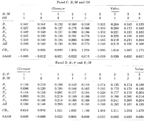
LSV test the contention that value strategies produce superior returns because investors extrapolate past performance too far into the future by examining simple one-variable classifications of glamour and value stocks. Glamour stocks are those that “have performed well in the past,” and “are expected by the market to perform well in the future.” Value stocks are those that “have performed poorly in the past and are expected to continue to perform poorly.” The stocks are classified on the basis of one of four variables: book-to-market (B/M, the inverse of price-to-book), cash flow-to-price (C/P), earnings-to-price (E/P), and 5-year average growth rate of sales (GS). LSV examine 2,700 firms on the NYSE and AMEX between 1968 and 1989. At the end of each April, they rank each stock on the basis of the variable tested (B/M, C/P etc) and then divide the stocks into deciles. Each decile is treated as a portfolio and held for 5 years. LSV track the performance of each decile portfolio in each of the 5 years and present the results as follows (Rt is the average return in year t over the 5 years after formation, CR5 is the compounded 5-year return assuming annual rebalancing. SAAR is the average annual size-adjusted return computed over the 5 years after formation. The Glamour portfolio is the decile portfolio containing stocks ranked lowest on B/M, C/P, or E/P, or highest of GS and vice versa for the Value portfolio):

As the four panels make clear, value outperforms glamour in rank order and regardless of the simple one-variable classification chosen. LSV attribute the outperformance to the failure of investors to formulate their predictions of the future without a “full appreciation of mean reversion.”

That is, individuals tend to base their expectations on past data for the individual case they are considering without properly weighting data on what psychologists call the “base rate,” or the class average. Kahneman and Tversky (1982, p. 417) explain:

One of the basic principles of statistical prediction, which is also one of the least intuitive, is that extremeness of predictions must be moderated by considerations of predictability… Predictions are allowed to match impressions only in the case of perfect predictability. In intermediate situations, which are of course the most common, the prediction should be regressive; that is, it should fall between the class average and the value that best represents one’s impression of the case at hand. The lower the predictability the closer the prediction should be to the class average. Intuitive predictions are typically nonregressive: people often make extreme prediction on the basis of information whose reliability and predictive validity are known to be low.

Anatomy of a Contrarian Strategy: LSV’s Two-Dimensional Classification

According to LSV, to exploit this flaw of intuitive forecasts, contrarian investors should sell stocks with high past growth as well as high expected future growth and buy stocks with low past growth and as well as low expected future growth.

Prices of these stocks are likely to reflect the failure of investors to impose mean reversion on growth forecasts.

LSV test the Two-Dimensional Classifications in a similar manner to the one-variable classifications above. At the end of each April between 1968 and 1989, 9 portfolios of stocks are formed. The stocks are independently sorted into ascending order in 3 groups (rather than deciles, for the obvious reason – 9 annual portfolios is easier to track than 100): 1. the bottom 30%, 2. the middle 40%, and 3. the top 30% based on each of two variables. The sorts are for 5 pairs of variables: C/P and GS, B/M and GS, E/P and GS, E/P and  B/M and B/M and C/P. Depending on the two variables used for classification, the Value portfolio either refers to the portfolio containing stocks ranked in the top group (3.) on both variables from among C/P, E/P, or B/M, or else the portfolio containing stocks ranking in the top group on one of those variables and in the bottom group (1.) on GS and vice versa for Glamour. (For the purposes of this post, I’m including only those examining B/M as one of the variables. The others are, however, well worth considering. Value determined on the basis C/P or E/P combined with GS produced slightly higher cumulative returns averaged across all firms for the period of the study. Interestingly, this phenomenon reversed in large stocks, with B/M-based strategies producing slightly higher cumulative returns in large stocks.):

These tables demonstrate that, within the set of firms whose B/M ratios are the highest (in other words, the lowest price-to-book value), further sorting on the basis of another value variable – whether it be C/P, E/P or low GS – can enhance returns. This is LSV’s Two-Dimensional Classification. LSV conclude that value strategies based jointly on past performance and expected future performance produce higher returns than “more ad hoc strategies such as that based exclusively on the B/M ratio.” The strategy is quite useful. It can be applied to large stocks, which means that it can be used to implement trading strategies for larger and institutional investors, and will continue to generate superior returns.

Next we examine Joseph D. Piotroski’s F_SCORE as a means for juicing P/B.

Read Full Post »

« Newer Posts - Older Posts »